Deep Dive - Light-PEFT

Your LoRA experiment can fit its trainable-parameter budget and still miss its GPU memory or latency budget. The profiler shows why: every batch still reads the frozen backbone, builds its activations, and evaluates every attention head and feed-forward coordinate. The previous chapter's hosted Tinker loop saves optimizer state, but freezing weights doesn't make their forward path disappear.

That leaves an adaptation decision: which dense coordinates can this task afford to lose, and what evidence will let you remove them without silently damaging quality? Dropping a LoRA rank makes the update smaller. It doesn't make the frozen matrix W smaller.

Light-PEFT, a parameter-efficient fine-tuning (PEFT) method, takes a deliberately sharp route. It spends a short prefix scoring heads, feed-forward dimensions, adapter modules, and adapter ranks, then physically removes the quiet coordinates before the longer fine-tuning run.^{[1]Reference 1Light-PEFT: Lightening Parameter-Efficient Fine-Tuning via Early Pruninghttps://aclanthology.org/2024.findings-acl.447/}

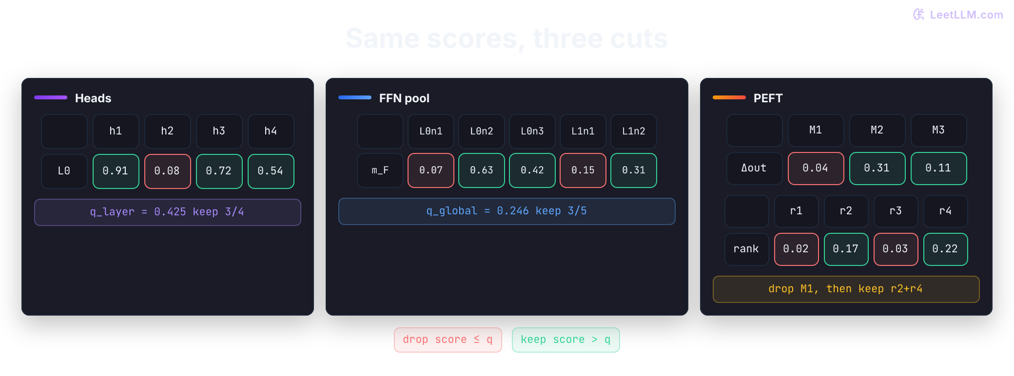
The handoff is the lesson. A cost ledger produces task-local scores, those scores become saved records, and only a checked record may become a physical slice. We'll use four heads, five FFN coordinates, and a rank-four adapter so each later cut has a visible owner.

We're reading the Association for Computational Linguistics (ACL) 2024 research release at the exact commit below, first inspected on September 23, 2026. On October 10, the repository's latest commit still matched that pin. Here ACL names the conference, not an access control list. The equations map onto NLU/estimate.py, NLU/train.py, and the bundled PEFT fork, not the current upstream PEFT API. Paper numbers stay inside their hardware protocol. A modern serving or reinforcement-learning system still has to prove the rest.^{[2]Reference 2Light-PEFT Source Repository at 7b10c22https://github.com/gccnlp/Light-PEFT/tree/7b10c22026fe6fa283d127353a50d6ed7176a8aa}

View larger

Start with cost that PEFT leaves behind

Before the notation, make a prediction. If the base weight is frozen and adapter rank r falls, which part of a token's path gets shorter? The low-rank branch does. The dense backbone path remains unless we change its shape.

Suppose a Transformer layer receives hidden states X. With ordinary LoRA, a frozen weight W receives a low-rank update:^{[3]Reference 3LoRA: Low-Rank Adaptation of Large Language Models.https://arxiv.org/abs/2106.09685}

where A maps from the hidden dimension to rank r, B maps back, and s is a scale. These equations use row-vector activations: A has shape [d_in, r] and B has shape [r, d_out]. PyTorch stores the transposes: lora_A.weight is [r, d_in] and lora_B.weight is [d_out, r]. Thus a rank cut removes mathematical A columns/B rows, or stored A rows/B columns. Only the adapter factors need optimizer updates. The layer still evaluates XW' for every token.

The phrase frozen describes parameter updates, not execution. Read one training step as a dependency chain:

1. Read frozen weights and trainable adapter weights.
2. Run forward through every surviving layer.
3. Keep activations or checkpoint enough information to reproduce them.
4. Backpropagate through the paths needed to reach trainable parameters, including frozen operations between adapters and loss.
5. Store gradients only for trainable parameters, then update the adapter.

PEFT removes a large optimizer and gradient burden. It doesn't automatically remove backbone FLOPs, backbone weight reads, or activation memory. The paper measures this directly: as OPT grows, forward time and peak memory rise even though LoRA avoids most backbone parameter gradients.^{[1]Reference 1Light-PEFT: Lightening Parameter-Efficient Fine-Tuning via Early Pruninghttps://aclanthology.org/2024.findings-acl.447/}

A tiny cost ledger

Use one layer with hidden size d = 8, sequence length S = 4, and a feed-forward width of 32. Before reading the table, predict what changing r can touch: the last row only. The rough dense projection count for one token is proportional to:

The adapter may add only a small number of trainable parameters, while the frozen 768 projection pairs per token still run. For S = 4, that's 3,072 projection multiply-accumulate pairs (6,144 FLOPs if one multiplication and one addition count separately). This excludes attention-score and value aggregation products, softmax, normalization, activation, and memory movement.

If a task never uses one attention head, or if many FFN coordinates carry little task signal, PEFT alone has no reason to skip them. A task-specific structured mask can make those coordinates absent from the second run.

Why quantization answers a different question

Quantization stores weights in fewer bits, reducing their storage footprint while kernels may dequantize values for computation. Quantizing a frozen base doesn't remove additional base optimizer state: ordinary LoRA already avoids that state. Structured pruning instead changes how many rows, columns, heads, or dimensions exist. Light-PEFT studies the second lever. The paper does not evaluate a QLoRA combination, so that configuration needs its own implementation and benchmark.^{[1]Reference 1Light-PEFT: Lightening Parameter-Efficient Fine-Tuning via Early Pruninghttps://aclanthology.org/2024.findings-acl.447/[4]Reference 4QLoRA: Efficient Finetuning of Quantized LLMshttps://arxiv.org/abs/2305.14314}

Before deleting base-model coordinates, identify what this repository supports and where a production integration needs its own evidence.

Research scope and production handoff

Before copying a pruning script into a training service, identify what you're holding. The source at commit 7b10c22026fe6fa283d127353a50d6ed7176a8aa is a small academic code release for the Findings of ACL 2024 paper. Its authors are Naibin Gu, Peng Fu, Xiyu Liu, Bowen Shen, Zheng Lin, and Weiping Wang. Their listed affiliations are the Institute of Information Engineering, Chinese Academy of Sciences, and the School of Cyber Security, University of Chinese Academy of Sciences.^{[1]Reference 1Light-PEFT: Lightening Parameter-Efficient Fine-Tuning via Early Pruninghttps://aclanthology.org/2024.findings-acl.447/}

Neither the paper nor repository names a company behind the project; primary ownership evidence points to those academic institutions and the gccnlp repository account.

Treat paper authors, the gccnlp repository account, and the GitHub contributors page as separate attribution records. The repository account publishes this snapshot; the contributors page reports code activity and does not map every paper author to a commit.^{[2]Reference 2Light-PEFT Source Repository at 7b10c22https://github.com/gccnlp/Light-PEFT/tree/7b10c22026fe6fa283d127353a50d6ed7176a8aa[5]Reference 5Light-PEFT Contributorshttps://github.com/gccnlp/Light-PEFT/graphs/contributors}

License wording needs the same care: the repository root has no repository-wide license file. The bundled peft/ subtree contains an Apache-2.0 LICENSE, and its setup metadata identifies that package as a PEFT fork. It's correct to call that subtree Apache-2.0 licensed. It's not correct to call the full Light-PEFT repository Apache licensed.^{[2]Reference 2Light-PEFT Source Repository at 7b10c22https://github.com/gccnlp/Light-PEFT/tree/7b10c22026fe6fa283d127353a50d6ed7176a8aa[6]Reference 6Apache License in Light-PEFT peft Subdirectoryhttps://github.com/gccnlp/Light-PEFT/blob/7b10c22026fe6fa283d127353a50d6ed7176a8aa/peft/LICENSE}

This distinction affects reuse. A research reader can inspect the code, paper, experiment settings, and history. A production team still needs a license review for every file, model checkpoint terms, dependency terms, and a maintenance plan. This checkout provides no service-level agreement, release cadence, or maintained model catalog. A useful handoff gives the production team a source map, an experiment receipt, and a clear account of the repository's research scope.

Repository maturity is equally narrow. There's no GitHub Actions workflow and no focused test suite for the Light-PEFT pruning path. The bundled peft/tests files exercise inherited configuration and adapter behavior, not the two-phase mask-to-surgery contract. Static Python compilation succeeds at the pinned commit, but that only proves files parse. It doesn't validate mask learning, tensor slicing, checkpoint restoration, or reported performance.^{[2]Reference 2Light-PEFT Source Repository at 7b10c22https://github.com/gccnlp/Light-PEFT/tree/7b10c22026fe6fa283d127353a50d6ed7176a8aa} That gap is useful context for the rest of the chapter: every claim that matters needs a file, shape, or measurement you can inspect.

Repository map: follow the handoff

The checkout is direct. It doesn't hide the two-phase boundary behind a package command. Read it by asking one question: what does estimate.sh produce that train.sh must consume?

Read the table from left to right: command, recorder, surgery helper, then consumer. This snapshot's custom model map registers RoBERTa sequence-classification and multiple-choice paths.

The paper evaluates LoRA and Adapter on RoBERTa-Large, OPT-1.3B, and OPT-6.7B, but the repository's runnable NLU path is much narrower than that sentence might suggest.^{[1]Reference 1Light-PEFT: Lightening Parameter-Efficient Fine-Tuning via Early Pruninghttps://aclanthology.org/2024.findings-acl.447/[2]Reference 2Light-PEFT Source Repository at 7b10c22https://github.com/gccnlp/Light-PEFT/tree/7b10c22026fe6fa283d127353a50d6ed7176a8aa}

Dependency age is part of the experiment

The release pins torch==2.0.1, transformers==4.31.0, datasets==2.13.0, numpy==1.25.1, scikit_learn==1.3.0, fairscale==0.4.13, and fsspec==2023.6.0. These versions describe the tested environment. Check current Transformers model classes, CUDA drivers, and PEFT APIs before reusing the code.

An environment receipt should carry the pinned commit, Python and CUDA versions, GPU model and memory, and an exact pip freeze or lock export. Add the dataset revision and preprocessing settings, random seed, command line for both phases, and hashes for saved mask and adapter files. Those fields let a later reader tell whether a changed result came from code, data, hardware, or a different mask.

Without those fields, a speed or accuracy number is hard to reproduce. Inspect the loaded model shapes after the second command to confirm it selected the intended reduced architecture.

Lifecycle: estimate, prune, continue

Light-PEFT separates estimation from physical pruning. During the first phase, masks and importance scores are trainable or recorded alongside PEFT updates. After a short prefix of training, the code selects survivors, slices tensors, writes records, and starts another trainer with those smaller tensors. The important handoff is this: a soft score becomes a shape-changing decision only after the saved records are checked.

View larger

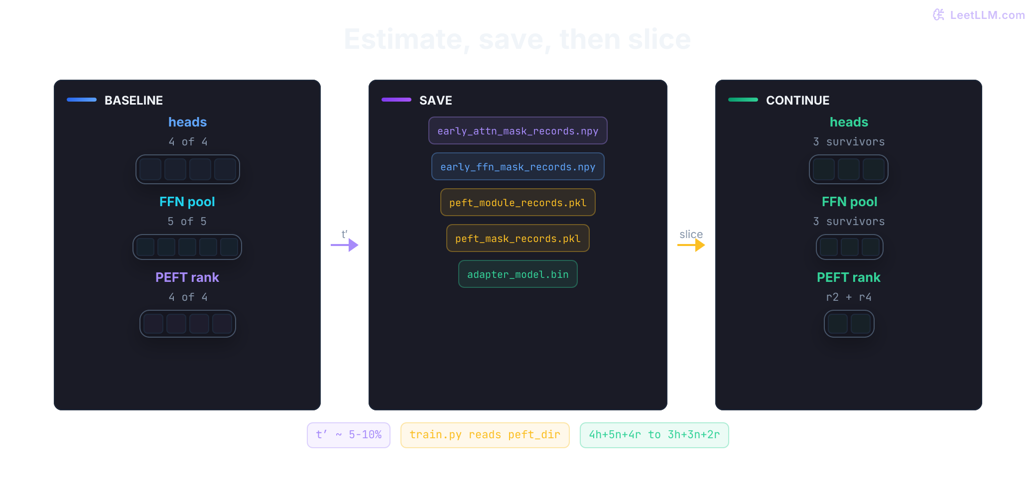
Let t be the full training step count and t′ the estimation prefix. For GLUE the paper keeps estimation around 5% of total steps; SuperGLUE stays within 10%; QA uses 10%. The appendix reports that extending estimation beyond about 6.8% didn't improve BoolQ.^{[1]Reference 1Light-PEFT: Lightening Parameter-Efficient Fine-Tuning via Early Pruninghttps://aclanthology.org/2024.findings-acl.447/}

The two shell scripts make that boundary visible. Read the diagram as a file handoff: estimate.sh learns evidence, peft_dir carries it, train.sh performs tensor surgery, and the new trainer receives a smaller model.

View larger

Those commands encode four handoffs:

1. Estimate. Build the baseline model and PEFT modules, initialize attention and FFN scalar masks to one, and train masks and PEFT parameters together for the estimation prefix.
2. Record. Evaluation and train-end callbacks save mask histories, PEFT module output ratios, and rank importance. Those records are the evidence that the next phase can inspect.
3. Slice and restore. The second process reads peft_dir, selects survivors, slices backbone and matching adapter feature dimensions, wraps the reduced base, restores filtered adapter weights, then slices adapter ranks. The estimate process owns the saved evidence; surgery consumes it.
4. Continue and measure. Start a new trainer with draw_and_training=True, then compare the complete wall-clock run, including estimation and continuation.

The mask is a score during phase one. A pruned dimension is a missing row or column during phase two. Before you run the second command, predict the failure if those rows and columns disagree: the adapter state can't fit the new base. For that reason, train.sh must use a compatible checkpoint and adapter state.

Masked Early Pruning of the foundation model

The first method narrows the cost question to the frozen Transformer: which coordinates contribute enough to justify running them? It doesn't guess individual weight values. It learns two trainable mask families, one scalar per attention head and one scalar per FFN intermediate dimension.

Attention head masks

Start with one attention layer. During estimation, every head still exists, but a scalar can turn its contribution up or down. If that scalar ends near zero, predict what happens next: the output is gated first; the head disappears only when the pruning helper slices its feature range.

Let layer i have N_H heads. A head output is multiplied by scalar m_A^(i). For one head:

When m_A is near zero, the head contributes little to the task loss under this early trajectory. The mask starts at one, so initial behavior matches the unmasked model. Gradient descent can move individual values, while an L1 term makes small values attractive. This signal applies to the current task and training trajectory; later training or tasks can change the head's value.

The repository implements this in models/hf_roberta/modeling_roberta.py. When config.mask_training is true, each attention block creates early_attn_mask shaped like (1, heads, 1, 1) and multiplies attention probabilities by it. At pruning time prune_heads builds an index of retained head coordinates and slices query, key, value, and output linear layers.^{[2]Reference 2Light-PEFT Source Repository at 7b10c22https://github.com/gccnlp/Light-PEFT/tree/7b10c22026fe6fa283d127353a50d6ed7176a8aa}

That slice is structured. It removes a whole head's feature range, not random individual weights. Tensor cores and framework kernels can see a smaller dense matrix. The score creates a candidate; the slice creates the possible steady-state saving.

FFN dimension masks

The FFN has a different shape contract. If one intermediate coordinate leaves, both projections around that coordinate must agree. Predict the bug if fc1 loses a column but fc2 still expects the old width: the next matrix multiplication won't line up.

An FFN block has an intermediate activation:

followed by a mask and the down projection:

Here m_F has one scalar per intermediate coordinate. In the source, early_ffn_mask is shaped like (1, intermediate_size). prune_inter_neurons slices intermediate.dense output rows and output.dense input columns using the surviving indices.^{[2]Reference 2Light-PEFT Source Repository at 7b10c22https://github.com/gccnlp/Light-PEFT/tree/7b10c22026fe6fa283d127353a50d6ed7176a8aa}

Removing an FFN coordinate therefore requires both sides of the bottleneck to agree. Slicing only fc1 leaves fc2 expecting the old width. Slicing only fc2 leaves an activation with a mismatched width. The helper changes both. Keep that paired-index rule in mind when you inspect a saved mask.

L1 penalty ranks candidate masks

The mask values still need a selection rule. A small value is a hint, not yet a deletion, so the mask trainer adds pressure toward sparse values:

trainer_base.py loops through attention and layer modules, sums the absolute values, and multiplies by l1_loss_coef. The shell example sets l1_loss_coef=1e-4. The paper's appendix reports λ_A = λ_F = 1 × 10^-4 for its main experiments.^{[1]Reference 1Light-PEFT: Lightening Parameter-Efficient Fine-Tuning via Early Pruninghttps://aclanthology.org/2024.findings-acl.447/[2]Reference 2Light-PEFT Source Repository at 7b10c22https://github.com/gccnlp/Light-PEFT/tree/7b10c22026fe6fa283d127353a50d6ed7176a8aa}

L1 doesn't decide an exact number of heads or neurons by itself. Ask what would happen if every mask stayed above zero: a later ratio and quantile would still choose survivors. L1 makes the score distribution easier to rank, then the requested ratio sets a capacity budget.

Layer-wise heads versus global FFN dimensions

Before choosing a threshold, decide who is allowed to compete. For attention heads, the helper defaults to layer-wise pruning. It computes a quantile separately within each layer, then prunes values at or below that layer's threshold. Every layer therefore loses roughly the requested fraction, subject to ties.

For FFN dimensions, train.sh passes --ffn_pruning_method "global". The helper accepts pruning_method="global", sets quantile_axis=None, and computes one threshold across all layers and dimensions. A layer with uniformly useful coordinates can keep more dimensions while another layer loses more. Global ranking spends the budget where scores are lowest; layer-wise ranking protects each layer's quota.

The repository uses layer-wise thresholds for attention heads and one global FFN threshold, so FFN dimensions compete across layers. Check score scales and survivor counts to confirm that this ranking matches the intended budget.

Also inspect the sign. The backbone masks are unconstrained trainable scalars, and prune_bert_attn and prune_bert_ffn threshold their signed recorded values, without taking magnitudes. Replace the walkthrough's 0.91 with -0.91: a 25% signed cut removes that head even though its gate magnitude is largest. Taking absolute values would instead remove the 0.08 head. A negative gate can reverse a contribution rather than make it quiet; changing the ranking rule is a method change, not a harmless numerical cleanup.^{[2]Reference 2Light-PEFT Source Repository at 7b10c22https://github.com/gccnlp/Light-PEFT/tree/7b10c22026fe6fa283d127353a50d6ed7176a8aa}

Random pruning as a control

get_early_model uses the saved mask arrays by default. With random_pruning=True, it creates seeded random scores and uses them in place of recorded values. Treat that branch as a control: it asks whether a claimed gain depends on task evidence rather than on any structured shape reduction.

Random pruning changes tensor shapes. Compare it with the same seed policy, ratio, hardware, and total time before attributing a performance gain to mask learning.

Multi-Granularity Early Pruning of PEFT

Once the backbone has candidate survivors, turn the same question toward the adapter. The second method sees adapter capacity at two scales. At module scale, should an entire LoRA or Adapter insertion remain at this weight or sub-layer? At rank scale, if it remains, how many of its low-rank coordinates are useful? A large module can barely change the task trajectory, while a small surviving module can still spend rank and compute.

Module removal can cut many small operations. Rank removal can retain a module while reducing its internal width. The paper reports both because increasing the number of structured modules can affect forward and backward time more than increasing the rank of one module under a fixed parameter budget.^{[1]Reference 1Light-PEFT: Lightening Parameter-Efficient Fine-Tuning via Early Pruninghttps://aclanthology.org/2024.findings-acl.447/}

Module importance from output change

Make the module decision from what it changes, not from its parameter count. If a module's output barely moves relative to the path it would have taken without the adapter, predict that its score will be close to zero.

For LoRA, the repository and paper compare the adapter output to the frozen weight output:

For an Adapter inserted after a sub-layer with output h:

An output ratio near zero says the module changed this task's activations little during the observed prefix. The code collects pos_importance_scores, averages the processed history, and writes peft_module_records.pkl.^{[1]Reference 1Light-PEFT: Lightening Parameter-Efficient Fine-Tuning via Early Pruninghttps://aclanthology.org/2024.findings-acl.447/[2]Reference 2Light-PEFT Source Repository at 7b10c22https://github.com/gccnlp/Light-PEFT/tree/7b10c22026fe6fa283d127353a50d6ed7176a8aa} The word observed matters: a quiet prefix can still hide a later task slice.

The displayed ratio suppresses implementation details: the fork's numerator includes LoRA scaling and dropout, its denominator includes the base linear bias, and MaskTrainer averages over non-padding tokens. There is no denominator epsilon in the forward ratio. The callback later replaces non-finite observations with zero, which can conceal instability and depress a module score. Log invalid counts before sanitization and report them alongside module scores.^{[2]Reference 2Light-PEFT Source Repository at 7b10c22https://github.com/gccnlp/Light-PEFT/tree/7b10c22026fe6fa283d127353a50d6ed7176a8aa}

The estimate places modules on all targeted weights so it can compare positions. This can cost more during the short prefix than a usual LoRA run. The paper's argument is that a small search cost can pay for a longer reduced run.

The helper prune_peft_modules takes module scores, computes a global quantile, and returns adapter parameter keys for surviving modules. get_early_peft_model filters the adapter state dict to those keys, sets reserved_modules, and enables prune_module so future wrapping skips removed positions.

Rank importance from first-order Taylor scores

Module pruning asks whether an insertion earns a place. Rank pruning asks which paired low-rank directions earn width. If setting one rank coordinate to zero would change the loss a lot, its first-order score should be large.

For parameter W_{i,j} in either down or up projection, the paper writes the first-order term as:

The paper's Equation 11 takes the absolute value of each weight-gradient product, then its rank score sums those magnitudes for one column of W_down and the matching row of W_up. This treats a rank coordinate as a unit. Removing only one side would break the low-rank product, so both matrices are sliced.^{[1]Reference 1Light-PEFT: Lightening Parameter-Efficient Fine-Tuning via Early Pruninghttps://aclanthology.org/2024.findings-acl.447/}

The repository makes a different aggregation choice. In MaskTrainer.training_step, each PEFT module computes weight * grad for its down and up matrices, averages along the complementary axis, takes absolute values of those means, stacks the two vectors, and sums them into importance_scores. Signed products can cancel before that absolute value: products [+2, -2] contribute zero through this mean, whereas the paper's sum of magnitudes gives four. The callback averages the later half of the history, replaces NaN and infinity with zero, multiplies by the absolute current mask when present, and writes peft_mask_records.pkl. A faithful port must choose which rule it reproduces.^{[2]Reference 2Light-PEFT Source Repository at 7b10c22https://github.com/gccnlp/Light-PEFT/tree/7b10c22026fe6fa283d127353a50d6ed7176a8aa}

The source's prune_peft_rank then computes a quantile across rank scores. For LoRA it slices lora_A rows and lora_B columns. If every rank is selected for removal, the module gets rank zero and its adapter is disabled. The same pattern exists for the bottleneck Adapter fork.^{[2]Reference 2Light-PEFT Source Repository at 7b10c22https://github.com/gccnlp/Light-PEFT/tree/7b10c22026fe6fa283d127353a50d6ed7176a8aa}

Layer-wise versus global adapter ranking

The helper accepts peft_pruning_method. A layer-wise choice computes a threshold inside each module. A global choice compares rank coordinates across all matching adapter modules. arguments.py defaults both ffn_pruning_method and peft_pruning_method to layerwise. The example train.sh overrides both to global. Predict the consequence before running: global rank pruning can spend most capacity in a few modules; layer-wise pruning computes a separate threshold per module. Record those flags in the receipt; copying only the ratios isn't enough.

Global rank pruning can concentrate capacity in a few modules. Layer-wise pruning sets separate thresholds, yet tied scores can still remove an entire module at a modest ratio. Check each resulting rank before export.

Tiny numerical walk-through

Now make the cuts by hand. Use four attention heads in one layer, with the same numbers as the score map above. Before reading the result, predict which head falls below a layer-wise 25% cut:

Request an attention pruning ratio of 0.25. With NumPy's default linear interpolation, the layer-wise 25th percentile is 0.425 for this tiny list. The source keeps values strictly above that threshold, so head 2 is removed and heads 1, 3, and 4 survive. Query, key, value, and output slices now use three head ranges instead of four. The useful distinction is visible: the threshold chooses head 2; the four synchronized slices make the choice physical.

Next, change the competition. Use five FFN coordinates across two layers and predict which two a global 40% cut removes:

For a global 40% pruning ratio, sort values: 0.07, 0.15, 0.31, 0.42, 0.63. Linear interpolation gives 0.15 + 0.6 × (0.31 − 0.15) = 0.246, removing two low coordinates and leaving 0.31, 0.42, 0.63. The five-coordinate pool is a small arithmetic example, not the rectangular unpruned RoBERTa mask layout. A global cut can remove several coordinates from one layer if that is where the low scores are.

For the adapter, let three LoRA insertions produce output ratios 0.04, 0.31, and 0.11. Predict the module cut first. A pruning ratio of 0.33 gives the threshold 0.04 + 0.66 × (0.11 − 0.04) = 0.0862, so the strict comparison removes the 0.04 module. For a surviving module, suppose rank scores are [0.02, 0.17, 0.03, 0.22] and rank pruning ratio is 0.50. The median threshold is 0.10, so ranks 2 and 4 survive in this local example. The adapter's down projection keeps the corresponding rows and its up projection keeps matching columns.

The arithmetic separates three decisions:

• a score says how much a coordinate changed the observed task trajectory;
• a quantile turns scores into a budget;
• a physical slice turns the budget into dense smaller tensors.

None of those steps says that a coordinate is universally unimportant. A new task, sequence distribution, adapter target set, or reward can rank it differently.

Code path from shell to saved artifacts

Now follow the handoff in the files. Before running anything, predict what the first command owns: it should create evidence, not a reduced model. The default scripts/estimate.sh pins one GPU (CUDA_VISIBLE_DEVICES=2 in the example), GLUE SST-2, RoBERTa-Large, LoRA rank 8, sequence length 128, batch size 32, five epochs, and max_steps=800. It passes --early_search True --use_mask_trainer True --use_peft True and writes under:

results/sst2/roberta-large-lora-p2-first_order/

That path depends on DATASET_NAME, model_name_or_path, adapter name, and peft_imp. The source's p2-first_order string controls how PEFT importance is recorded. It isn't a generic method name recognized by current PEFT releases.

What estimate.py records

At on_train_begin, SuperGLUECallback creates one list per encoder layer for attention and FFN masks. It also writes init_peft_mask_records.pkl with initial PEFT mask tensors. The callback is establishing the history that later pruning will treat as evidence.

At each evaluation, the callback records current mask values. At train end it records one final value, stacks each layer's history, and saves:

early_attn_mask_records.npy
early_ffn_mask_records.npy

It also processes each PEFT module's score history. The code averages the latter half of the history, sanitizes NaN and infinity, and writes:

peft_module_records.pkl
peft_mask_records.pkl

These files are small relative to the model, but they are part of the run's provenance. Hash them and keep the seed with the command. If those files are missing or point to another run, the second phase has no trustworthy handoff.

What train.py reads

The second command consumes that handoff. The default scripts/train.sh points peft_dir at the estimate output and sets:

attn_pruning_ratio=0.333333333
ffn_pruning_ratio=0.333333333
module_pruning_ratio=0.75
rank_pruning_ratio=0.5
ffn_pruning_method=global
peft_pruning_method=global

Read those knobs in two groups. The ratios request how much to remove; the method flags decide which scores compete. This command asks for a 75% module cut and a 50% rank cut among surviving modules, then lets global FFN and rank thresholds spend those cuts across layers. Keep the ratios but switch to layer-wise ranking and you've run a different experiment.

It passes --draw_and_training True --use_peft True. The script-default ratios differ from Table 1: the paper's 72% retained LoRA row prunes 5/16 of the heads (0.3125) and 1/3 of the FFN dimensions. To reproduce that row, set the matching ratios explicitly; train.sh currently requests a 75% module cut and a 50% rank cut.

The three supplied scripts use different datasets and training policies, so their default wall times cannot serve as a matched pruning benchmark. vanilla_train.sh selects MNLI, five epochs, query/value LoRA targets, warmup_ratio=0.06, and weight_decay=0.1. The estimate and continuation scripts select SST-2, target query/key/value plus attention and FFN dense projections, and continue for ten epochs after the 800-step estimate. Align dataset and revision, target policy, optimizer settings, and total training budget before timing a local baseline.^{[2]Reference 2Light-PEFT Source Repository at 7b10c22https://github.com/gccnlp/Light-PEFT/tree/7b10c22026fe6fa283d127353a50d6ed7176a8aa}

get_trainer.py calls get_early_model, which loads the two .npy arrays, chooses the final recorded step, and prunes RoBERTa heads and FFN dimensions. get_early_peft_model then loads adapter state, selects modules, slices adapter feature dimensions to match the reduced base, wraps that base, restores filtered weights, and finally prunes ranks. Rank and module pickle reads are conditional on nonzero pruning ratios.^{[2]Reference 2Light-PEFT Source Repository at 7b10c22https://github.com/gccnlp/Light-PEFT/tree/7b10c22026fe6fa283d127353a50d6ed7176a8aa}

Partial rank pruning changes actual A/B tensor shapes without updating the module's nonzero r or recomputing scaling. The original scale therefore survives the slice. Rebuilding a modern adapter with alpha/new_rank would change its output. Export and reload need explicit per-module shapes and scale alongside the original configuration. Also treat .pkl files and the old torch.load checkpoint path as trusted-code inputs: don't load artifacts from an untrusted source.

The second command isn't a resume in the optimizer sense. It constructs a new model and trainer after tensor surgery. set_mask(init_mask=False) resets surviving backbone masks to one and disables their training/forward gates. The saved scalar magnitudes select coordinates; they aren't preserved as learned gates in continuation. If you need an uninterrupted optimizer trajectory, this code isn't that path.

Failure modes at the estimate-to-train handoff

If estimation succeeds but continuation fails, classify the boundary before changing a ratio. A missing record points backward to the producer; a shape error points forward to the surgery and state pairing. The table gives each symptom a first check:

For a concrete diagnosis, suppose all four record files exist but train.py raises an adapter-key mismatch. Don't lower the pruning ratio first. Compare the base revision, target module list, and surviving shapes with the estimate receipt; the producer and consumer disagree about identity or layout. A linear shape error points to the same handoff after surgery, while a missing .npy points back to the estimate output path.

Keep command output in a receipt. The printed "pruning complete" line records that control flow reached the helper. Verify shape correctness, run a batch, and measure the complete path to assess throughput and task quality.

A copy-runnable mask simulator

The following standard-library example lets you test the score-to-index handoff without a GPU. Before running it, predict three things: the head threshold should keep indices [0, 2, 3], the global FFN cut should keep [1, 2, 4], and every retained rank should appear in both adapter projections. The example mirrors score selection, strict > thresholding, and rank pairing without importing Torch or NumPy. It doesn't emulate Transformer kernels. Its value is the invariant: every retained rank is present in both adapter projections, and every selected backbone coordinate is explicit.

from dataclasses import dataclass
from math import isfinite

def quantile(values, ratio):
    ordered = sorted(values)
    if not ordered or not isfinite(ratio) or not 0 <= ratio <= 1:
        raise ValueError("need scores and a finite ratio in [0, 1]")
    if not all(isfinite(value) for value in ordered):
        raise ValueError("scores must be finite")
    position = (len(ordered) - 1) * ratio
    low = int(position)
    high = min(low + 1, len(ordered) - 1)
    fraction = position - low
    return ordered[low] + fraction * (ordered[high] - ordered[low])

def keep_above(scores, ratio):
    threshold = quantile(scores, ratio)
    return threshold, [index for index, score in enumerate(scores) if score > threshold]

@dataclass(frozen=True)
class RankPair:
    down_row: int
    up_column: int

heads = [0.91, 0.08, 0.72, 0.54]
ffn = [0.07, 0.63, 0.42, 0.15, 0.31]
rank_scores = [0.02, 0.17, 0.03, 0.22]

head_threshold, kept_heads = keep_above(heads, 0.25)
ffn_threshold, kept_ffn = keep_above(ffn, 0.40)
rank_threshold, kept_ranks = keep_above(rank_scores, 0.50)
rank_pairs = [RankPair(index, index) for index in kept_ranks]

assert kept_heads == [0, 2, 3]
assert kept_ffn == [1, 2, 4]
assert [pair.down_row for pair in rank_pairs] == [1, 3]
assert [pair.up_column for pair in rank_pairs] == [1, 3]
assert keep_above([1, 1, 1, 1], 0.25)[1] == []
# This is the raw threshold helper. The upstream caller skips ratio=0.
assert keep_above(heads, 0)[1] == [0, 2, 3]
assert keep_above(heads, 1)[1] == []
signed_heads = [-0.91, 0.08, 0.72, 0.54]
assert keep_above(signed_heads, 0.25)[1] == [1, 2, 3]
assert keep_above([abs(score) for score in signed_heads], 0.25)[1] == [0, 2, 3]

print(f"heads threshold={head_threshold:.3f} keep={kept_heads}")
print(f"ffn threshold={ffn_threshold:.3f} keep={kept_ffn}")
print(f"rank threshold={rank_threshold:.3f} pairs={rank_pairs}")

heads threshold=0.425 keep=[0, 2, 3]
ffn threshold=0.246 keep=[1, 2, 4]
rank threshold=0.100 pairs=[RankPair(down_row=1, up_column=1), RankPair(down_row=3, up_column=3)]

The output checks the simulator's logic. Its quantile is a transparent teaching implementation; the repository uses NumPy's behavior. For a production reproduction, compare exact selected indices against NumPy before using a trainer helper.

Try changing the rank ratio to 0.75. The retained pair list shrinks, but every pair still has matching down and up coordinates. Try changing one backbone score to a tie at the threshold. The strict comparison then makes the survivor count depend on the quantile value.

Verify the adapter product and task behavior

The next standalone CPU example uses PyTorch's stored orientation without importing PyTorch. It tests every subset of a rank-four adapter. A physically sliced product must equal a full-width product with the removed rank activations zeroed, at the same scale. This checks tensor algebra; evaluate model output and task accuracy separately.

from itertools import combinations

def linear(weight, vector):
    return [sum(w * x for w, x in zip(row, vector, strict=True)) for row in weight]

A = [[1, 2, 0], [0, 1, 3], [2, 0, 1], [1, -1, 2]]  # [r, d_in]
B = [[1, 2, 3, 4], [-2, 1, 0, 3]]                    # [d_out, r]
x = [2, -1, 3]
hidden = linear(A, x)
checked = 0
for size in range(5):
    for kept in combinations(range(4), size):
        sliced_A = [A[k] for k in kept]
        sliced_B = [[row[k] for k in kept] for row in B]
        sliced = linear(sliced_B, linear(sliced_A, x))
        masked = linear(B, [value if k in kept else 0 for k, value in enumerate(hidden)])
        assert sliced == masked
        checked += 1

# Mismatching B's rank columns keeps valid shapes but changes the function.
correct = linear([[row[k] for k in [1, 3]] for row in B], [hidden[1], hidden[3]])
wrong = linear([[row[k] for k in [0, 2]] for row in B], [hidden[1], hidden[3]])
assert correct != wrong
original_scale, rebuilt_scale = 16 / 4, 16 / 2
assert [original_scale * y for y in correct] != [rebuilt_scale * y for y in correct]
print(f"paired subsets checked={checked}; mismatched pairing and scale changes detected")

paired subsets checked=16; mismatched pairing and scale changes detected

Neither example runs a Transformer, learns masks, checks an exported checkpoint, or reproduces GPU timings. The upstream helper also needs explicit guards for empty survivor sets and invalid histories. In particular, its random rank branch constructs an array and subsequently treats it like a name-keyed dictionary; the module helper accepts random_shuffle but doesn't use it. Don't interpret those flags as a validated end-to-end random control.^{[2]Reference 2Light-PEFT Source Repository at 7b10c22https://github.com/gccnlp/Light-PEFT/tree/7b10c22026fe6fa283d127353a50d6ed7176a8aa}

Paper evidence: read numbers with their boundary

Now separate the questions a benchmark can answer. The paper validates Light-PEFT on GLUE, SuperGLUE, and question-answering tasks. Its foundation models are RoBERTa-Large, OPT-1.3B, and OPT-6.7B. Its PEFT structures are LoRA and Adapter. These combinations define the published test scope; validate other models and adapters separately.^{[1]Reference 1Light-PEFT: Lightening Parameter-Efficient Fine-Tuning via Early Pruninghttps://aclanthology.org/2024.findings-acl.447/}

Table 1 trade-off

Table 1 compares LoRA on RoBERTa-Large with Light-PEFT variants. Before reading the numbers, predict what a faster row has to give up or account for: search overhead, retained capacity, or task score. Read each row as one quality, capacity, and timing choice. The values below pair paper-reported averages with speeds measured on the paper's test setup. Re-run the timing on the hardware and implementation you plan to use.

The average covers the paper's MNLI, QNLI, QQP, and SST-2 columns. Training speed includes estimation before pruning, measured on a single NVIDIA TITAN RTX 24GB GPU with batch size 32 and sequence length 128. The paper does not report an end-to-end download-to-export stopwatch. The 72% row prunes 5/16 of the heads and 1/3 of the FFN intermediate dimensions, then also prunes PEFT modules and ranks.^{[1]Reference 1Light-PEFT: Lightening Parameter-Efficient Fine-Tuning via Early Pruninghttps://aclanthology.org/2024.findings-acl.447/}

Notice the trade: the 67% retained configuration uses the same rounded 0.3M trainable parameter count as the 72% configuration, but gives up 0.3 GLUE average points for the reported 0.2× additional speedup. The useful comparison is a Pareto choice under a declared task and budget. "More pruning is always better" isn't a conclusion the table can support.

Relative to baseline LoRA, those rows lose 1.1 and 1.4 average accuracy points. The paper reports MNLI's matched validation accuracy and accuracy for the other three tasks. Appendix Table 7 supplies rank 8, 75% module pruning, 50% rank pruning, learning rate 3e-4, and task-specific estimation steps and epochs. It reports no repeated-run variance, confidence interval, or complete precision, warmup, synchronization, and timing receipt. Use the speed ratios as reported measurements under that setup; reproduce the measurement before relying on them for a deployment decision.^{[1]Reference 1Light-PEFT: Lightening Parameter-Efficient Fine-Tuning via Early Pruninghttps://aclanthology.org/2024.findings-acl.447/}

Figure 4 training cost

The mechanism makes a second prediction: if physical widths shrink, model-weight memory and activation memory should both fall, while the size of the fall still depends on the workload.

Figure 4 measures RoBERTa-Large on an NVIDIA RTX 3090 with batch size 32 and sequence length 128. In that experiment, the Light-PEFT setting retains 67% of foundation parameters and 0.3M trainable parameters. The paper reports 32% lower model-weight memory, 40% lower activation memory, and 39% lower peak memory. Its ten-batch forward and backward timing is 2.2× faster than baseline LoRA.^{[1]Reference 1Light-PEFT: Lightening Parameter-Efficient Fine-Tuning via Early Pruninghttps://aclanthology.org/2024.findings-acl.447/}

The peak-memory result follows the mechanism taught earlier. Removing dimensions reduces both weight storage and intermediate activation shapes. The 2.2× ratio comes from the reported ten-batch forward/backward run on this configuration. Batch size, sequence length, GPU, and implementation affect the ratio; measure those settings again on your target workload.

Table 5 inference boundary

Hold the foundation at 52% retained and look at the module column. What can change the inference row without changing that backbone? The number of surviving adapter insertions. Section 5.3.2 places the efficiency experiments on an RTX 3090; Table 5 uses OPT-6.7B with batch size 96 and maximum length 100. It reports load memory and inference speed for foundation pruning and optional module pruning.

The paper therefore reports up to 1.6× inference speed and 48% lower load memory in this OPT-6.7B protocol. "48%" compares 6.5G with 12.5G approximately, and the 1.6× row also removes 75% of PEFT modules. Keep those axes together when reproducing the result.^{[1]Reference 1Light-PEFT: Lightening Parameter-Efficient Fine-Tuning via Early Pruninghttps://aclanthology.org/2024.findings-acl.447/}

What the paper leaves untested

The paper evaluates those combinations. Validate support and benefit separately for:

• modern frontier MoE post-training;
• multi-task adapter fleets sharing one base;
• online reinforcement-learning distribution shifts;
• QLoRA plus Light-PEFT combinations;
• distributed large-scale jobs with tensor, pipeline, or expert parallelism;
• current CUDA, ROCm, or accelerator kernel stacks;
• continual pruning while adapters are loaded per request.

A capability claim beyond that scope needs a model-specific implementation, loader test, benchmark protocol, and license check.

Permanent base masks change serving semantics

Training has handed us a shape-specific artifact. Imagine a compiled plan for 16 heads receiving a 12-head pruned base. Can the server reuse its cached tensors? No. A shared-base adapter service relies on compatible base dimensions and coordinate identities. Ordinary multi-adapter serving makes the same bet: request A selects adapter A, request B selects adapter B, and both still fit the same frozen matrix dimensions. A structured Light-PEFT run physically removes heads and FFN coordinates from that base.

That creates a serving choice:

The paper's "plug-and-play" claim covers switching masks and PEFT modules in its tested setup.^{[1]Reference 1Light-PEFT: Lightening Parameter-Efficient Fine-Tuning via Early Pruninghttps://aclanthology.org/2024.findings-acl.447/} Serving arbitrary adapters from one production base requires a deployment-specific implementation and kernel plan. Make that decision after defining the slice, because it determines which artifacts can share a shape.

KV caches and compiled kernels add more state. A cache keyed only by model name and adapter ID can return incompatible tensors if the base shape or pruning seed changes. Include base revision, shape signature, selected-coordinate identity, and adapter revision in cache keys. Two slices can have identical dimensions but retain different original heads. The cache key is part of the pruning contract, not an implementation detail to fill in later.

Reinforcement-learning distribution shifts

Early scores come from a prefix of one data distribution. Ask whether that evidence is still valid after the model changes. In supervised fine-tuning, later batches can already differ from the prefix. In online RL, the policy changes the data it receives, so the shift can be stronger:

1. The initial policy samples trajectories from distribution D_0.
2. Early masks rank coordinates using rewards and gradients from D_0.
3. Pruning changes policy capacity and removes some routes.
4. The new policy samples D_1, which can contain states absent from D_0.
5. A removed head or FFN coordinate may be important in D_1 even if it looked quiet in D_0.

The paper's static GLUE and QA protocol does not measure this RL concern. An RL evaluation should log policy version, mask version, trajectory distribution, reward slices, and divergence before and after pruning. A held-out online stream can test whether reward collapse follows the physical cut. The important question is causal: did the reward change because of the physical cut, or because the policy changed the data?

If a system needs reversible exploration, keep the unpruned base or a set of checkpoints. A one-way physical slice is cheap to run but expensive to undo without rebuilding the original model.

Operational fragility and safe experiment design

The code is concise because it assumes a controlled research machine. A production adaptation fails at handoffs, not at the idea's headline: a state dict can have familiar keys and still target the wrong shapes, or a speedup can disappear once estimation is counted. Treat each contract below as a gate.

Shape contract

Before loading adapter state, predict the failure from one mismatched dimension, then verify:

• base model identifier and revision;
• number of layers;
• surviving attention heads per layer;
• hidden size and head dimension;
• surviving FFN width per layer;
• target module names;
• LoRA rank or Adapter bottleneck width;
• bias and dropout configuration.

The source slices tensors in place and restores state dict entries by name. A different Transformers implementation can rename a module or store transposed weights. A name match isn't enough; compare tensor shapes before the load. If the shape signature changes, stop before the adapter can fail deeper in the forward pass.

Numerical contract

Mask penalties and first-order scores depend on gradients. A score change can come from numerical settings rather than task evidence, so record:

• precision and autocast state;
• loss scale if mixed precision is enabled;
• gradient clipping;
• learning rate and mask learning-rate multipliers;
• NaN and infinity counts;
• evaluation interval used to sample mask history.

The repository uses separate attention and FFN mask learning-rate coefficients. MaskTrainer has constructor defaults of 100 and 50, but get_trainer.py passes arguments.py values, and those dataclass defaults are both 1. The example shells don't override them. A port that silently keeps the constructor defaults, or changes the multipliers, changes the search problem.^{[2]Reference 2Light-PEFT Source Repository at 7b10c22https://github.com/gccnlp/Light-PEFT/tree/7b10c22026fe6fa283d127353a50d6ed7176a8aa} Record the resolved values passed to the trainer; constructor defaults alone can mislead.

Measurement contract

A speed claim can be true and still answer the wrong question if the stopwatch starts after the expensive search. Time the complete workflow:

clean process start
  + model and tokenizer load
  + dataset preparation
  + estimation prefix
  + mask and score serialization
  + physical pruning and model rebuild
  + continued fine-tuning
  + evaluation and export

The paper's Table 1 explicitly includes estimation before pruning. A benchmark that starts its stopwatch after the masks exist will overstate speedup. A benchmark that includes data download but not model load will answer a different question. State both wall-clock definitions.

Failure isolation

Run checks in dependency order:

1. Environment and baseline. Import the pinned dependency set, load the tokenizer and base model without PEFT, then run one baseline forward and backward batch.
2. Estimation. Run one estimation batch, inspect mask ranges, and confirm all four record files exist.
3. Surgery. Rebuild one pruned model, print its shapes, and restore one filtered adapter state dict.
4. Smoke test. Run one post-pruning batch. Only then start the full continuation.

This order separates environment errors from score errors and shape errors. It also avoids burning a long GPU job before discovering that the saved peft_dir points to another dataset. Those gates are about this repository. They don't say how the same idea differs from LoRA or QLoRA, which leave the base shape alone.

Scope comparison with nearby methods

The difference is the dense shape. Light-PEFT combines pruning with PEFT. It isn't a replacement name for every efficient fine-tuning approach.

Light-PEFT's efficiency comes from paying for a change in the model's dense shapes. That makes its steady-state run different from a method that only gates execution or stores lower-precision weights. Because the method rewrites dense dimensions, its runtime must accept the resulting shape.

Questions to ask before adapting the code

When moving beyond RoBERTa NLU, use these as go-or-stop questions in order. A “yes” at one gate doesn't imply a “yes” at the next.

Does the model expose the same structures?

The code knows RoBERTa attention and layer classes. A decoder-only model may store fused QKV, grouped-query heads, rotary embeddings, parallel residual paths, or gated FFN matrices. A head slice must respect those layouts. An MoE layer adds expert routing and capacity rules that this code doesn't model.

Can a global score compare coordinates?

Global FFN and rank quantiles assume scores share a meaningful scale. Layer normalization, module placement, and gradient scale can make one layer's numbers incomparable. Normalize or keep thresholds local only after checking the score distribution.

Is physical pruning legal for the deployment runtime?

A training fork can slice PyTorch linear layers. A fused inference engine may require a separate kernel for each head count, tensor-parallel shard, or expert layout. Prove that the loader, compiler, quantizer, and serving cache all understand the new shape.

Does the task distribution stay stable?

Static labels and online rewards answer different questions. For multi-task or RL use, hold out shifts and re-evaluate after every pruning boundary. Early importance isn't a lifetime contract.

Can the experiment be undone?

Keep original base weights, original adapter state, selected indices, and a manifest. A mask vector alone can't reconstruct removed matrix rows unless the original checkpoint remains available.

What a pruning review must defend

A credible review should connect the repository's choices to an artifact that another engineer can inspect:

• Separate trainable-state savings from frozen projection, activation, and attention costs; count estimation before claiming a training speedup.
• Trace the exact commit from score history through selected coordinate indices, adapter feature slicing, restoration, and rank slicing. Explain the stored A/B orientation and preserved scale.
• Report per-layer head and FFN survivors, per-module rank shapes, non-finite score counts, and a post-pruning batch result. A ratio or a successful load alone isn't enough.
• Keep paper-reported timings separate from local measurements, and distinguish the four-task GLUE average from a full-suite score.
• Name the deployment's base revision, selected coordinates, compatible adapters, rollback artifact, and unresolved license or runtime constraints.

Follow-up questions

Mastery quiz

Course complete: Return to the curriculum roadmap. A frozen backbone still costs a forward pass, and a mask becomes a shape change only after the saved records are checked. The same habit applies to the earlier project chapters: pin the commit, test the claim, and keep a receipt. For a career next step, turn those receipts into portfolio evidence with AI Engineer Portfolio Projects That Get Interviews.