Data Structures for AI

In our tiny corpus, a user searches for red fox. Document 2 contains both words, document 0 contains one, and document 1 contains neither:

A loop over a Python list can find those matches. You used lists and dictionaries in Python for AI Engineering: lists keep items in order, while dictionaries retrieve values by key. Here the choice changes how much work a search repeats. A retriever finds documents relevant to a query; ours will rank them by the number of distinct query words they contain.

With three notes, scanning every word is cheap. With many notes and repeated queries, we'd rather build a lookup once and reuse it. The same records will help us compare lists, indexes, heaps, and caches without changing the search problem.

Let the operation choose the shape

Before naming a structure, ask which operation must stay cheap and predictable:

• "Which item is at position 2?" points to a sequence.
• "Which documents contain red?" points to a key-value mapping.
• "Have I already seen document 2?" points to a set.
• "Which waiting job is oldest?" points to a queue.
• "Which retained result is weakest?" points to a heap.
• "Which notes share a parent topic, link to each other, or begin with this prefix?" points to a tree, graph, or trie.

These aren't interchangeable labels. Each structure preserves a different promise about position, identity, order, or connection. The useful choice follows from the operation you need to repeat.^{[1]Reference 1Introduction to Algorithms (3rd ed.)https://mitpress.mit.edu/9780262033848/introduction-to-algorithms/}

Lists and array-shaped sequences

A Python list is an ordered, mutable sequence. CPython stores it as a resizable array of object references, so an integer index reaches a known position directly. Our strings fit a list because they're ordinary Python objects.^{[2]Reference 2Python Design and History FAQhttps://docs.python.org/3/faq/design.html}

That shape differs from array.array, which packs a restricted basic value type, and from a NumPy array or tensor, which usually holds one numeric type in a rectangular shape and supports vectorized math. The distinction matters here because the corpus needs flexible Python objects, not a rectangular block of one numeric type.

Start with three operations and predict what each one has to move:

An append occasionally needs a larger backing array and copies existing references. Spread across many appends, that occasional resize still gives constant work per append on average. The complexity table calls this amortized constant time.

That last row explains why a list is a poor first-in, first-out queue when code repeatedly uses pop(0). The output is correct, but removing the first item still moves every later reference. When arrival order becomes the operation to protect, a deque fits better. We'll use it later.

The list is still the right starting point here because document order is stable and a complete scan is easy to verify by hand.

Now run the query against the list. The match counts look like this:

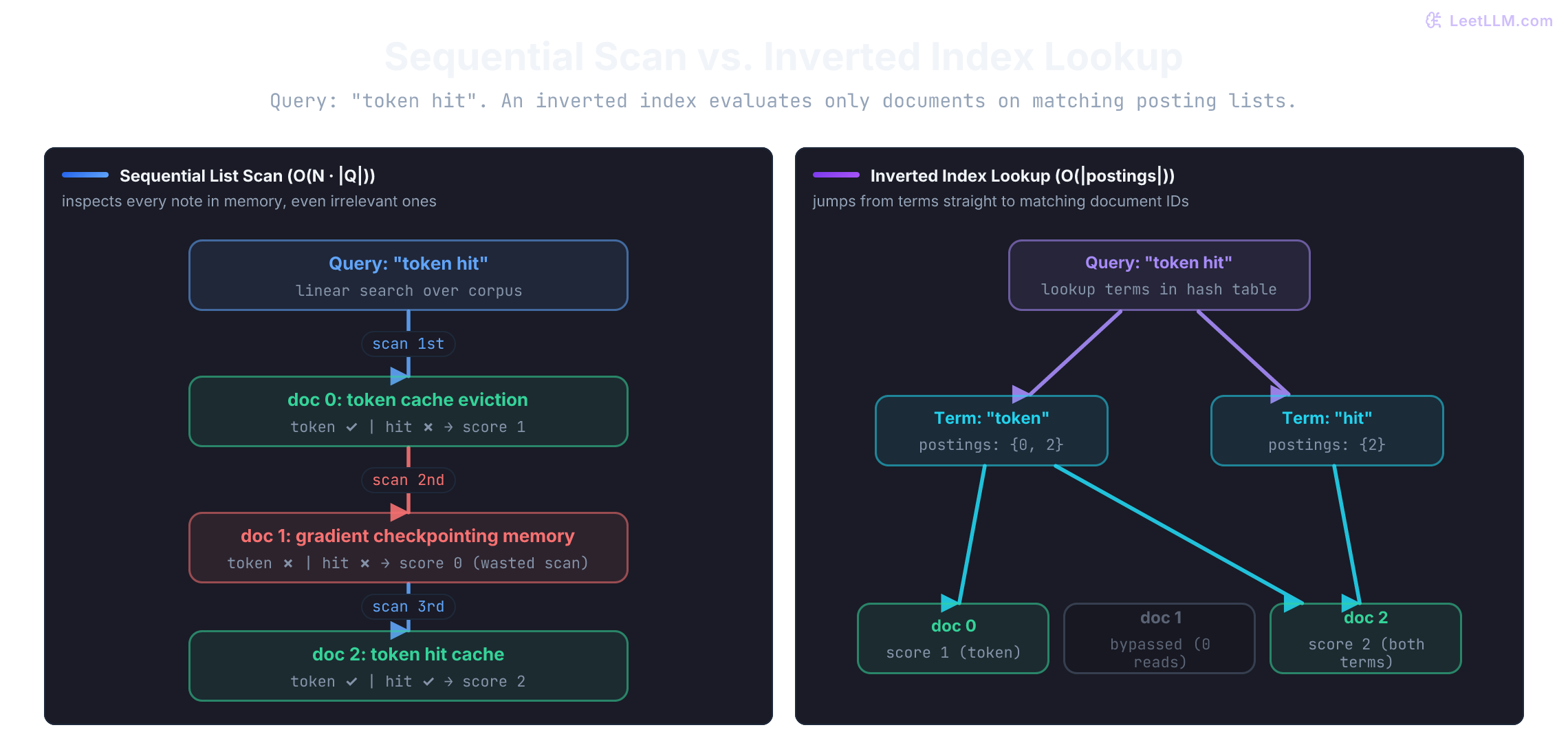
Document 2 should rank above document 0 because it matches both terms. Document 1 contributed nothing, yet the scan still opened it. That unused read is the cost we want the next structure to remove.

To skip irrelevant documents, we'll need extra information prepared before the query arrives. That saves repeated scanning, at the cost of storing and updating an index.

Building an inverted index

The query starts with a term such as red, so let the lookup start there instead of at document 0. The system should jump from the term to matching documents.

An inverted index answers that direction of lookup. It reverses the document-to-terms view into a term-to-documents map. The key changes from a document ID to the thing the query already has: a term.

Python calls its built-in hash map a dict. A hash function narrows down where a key could be stored; equality checks distinguish keys that collide. Keys must be hashable: their hash stays stable, and keys that compare equal must have equal hashes. Strings and integers work as keys; a mutable list doesn't.^{[3]Reference 3Built-in Typeshttps://docs.python.org/3/library/stdtypes.html}

Python dictionaries preserve insertion order, but that order isn't what makes lookup fast. For this index, the important behavior is that a term leads to its posting collection, regardless of where that key was inserted.

The hash narrows the lookup; it isn't a document identity. Two unequal keys can have the same hash and still occupy separate dictionary entries. Keep the original term as the key, not hash(term). Likewise, our document IDs are list positions only because this corpus keeps its order. Removing doc 0 would shift later positions and invalidate existing postings. A changing corpus needs stable document IDs or a rebuilt index.

The index maps each term to its posting list. A posting records a matching document ID; larger indexes can also store term positions or frequency. In this first version, a Python set[int] is enough because our score asks only whether each query term appears in each document.^{[4]Reference 4Introduction to Information Retrieval.https://nlp.stanford.edu/IR-book/}

Build the index by hand

Split each document into terms and store the matching document IDs. For red, predict which rows should be reachable before checking the table:

Now the query can enter through the index. It asks for two posting lists instead of reopening all three documents:

Turn those posting lists into match counts by adding one for each query term that contains a document:

Document 2 wins because it matches both terms. Document 0 still matters because it matches one term. The index removed document 1 from scoring entirely, so lookup and scoring now have a visible boundary.

View larger

Why a set lives inside the dictionary

The dictionary solves exact term lookup. The set solves uniqueness and membership. Keeping those jobs separate makes the index easier to reason about.

Suppose document 2 were red red fox. The posting list for red should still contain document 2 once, not twice. That's why the value is a set of document IDs instead of a list of document IDs.

Keep the two operations separate:

• Dictionary asks: "given this term, which collection is its value?"
• Set asks: "is this document ID already in that collection?"

Python sets don't promise a useful iteration order, so examples sort them before printing. Production lexical indexes commonly keep ordered, compressed posting lists and richer statistics. The Python set is a teaching choice: it makes membership and duplicate prevention visible before storage layout and fast posting intersections enter the design.^{[4]Reference 4Introduction to Information Retrieval.https://nlp.stanford.edu/IR-book/}

A repeated term is the smallest proof. In the demo below, document 2 says red twice, but membership in the red posting set still contributes one document ID.

from collections import defaultdict

docs_with_repeat = [
    "red bird sings",
    "blue whale swims",
    "red red fox",
]
postings: dict[str, set[int]] = defaultdict(set)

for doc_id, text in enumerate(docs_with_repeat):
    for term in text.split():
        postings[term].add(doc_id)

print("red postings", sorted(postings["red"]))
print("document 2 counted once", len(postings["red"]) == 2)

red postings [0, 2]
document 2 counted once True

Keep only the winners

The index has narrowed the query to scored candidates. Now the system needs the best few results, not a fully sorted report of the corpus. That distinction determines the next structure.

A heap maintains a small group of winners while candidates arrive. If you need two results out of thousands, it can avoid fully sorting candidates you won't return. With only two matches in our current corpus, a sort is perfectly reasonable; add one more candidate to expose the selection decision.

For the three notes, the scored candidates are:

A binary heap stores a partial order rather than a fully sorted list. The heapq operations used here maintain a min-heap: the smallest key is always at index 0. The remaining list isn't globally sorted, which is fine because the root is the only position we need to inspect for eviction.^{[5]Reference 5heapq: Heap queue algorithmhttps://docs.python.org/3/library/heapq.html[1]Reference 1Introduction to Algorithms (3rd ed.)https://mitpress.mit.edu/9780262033848/introduction-to-algorithms/}

That root guarantee fits top-k retrieval. Keep only k winners, with the weakest winner at the root. You often want the best 5, 10, or 20 candidates rather than a complete ranking of every candidate. The root tells you exactly which retained result can leave when a stronger candidate appears.

Suppose doc 3, red fox runs, arrives with score 2. Keep only two results. Doc 0 should leave because its score is 1, while docs 2 and 3 each score 2. Which tied result should come first?

Use keys (score, -doc_id). Python compares tuples from left to right, so score wins first. When scores tie, doc 2 has key (2, -2), which is larger than doc 3's (2, -3). The lower document ID wins the tie. Inside a min-heap, however, the smaller key goes at the root so it's ready for eviction:

View larger

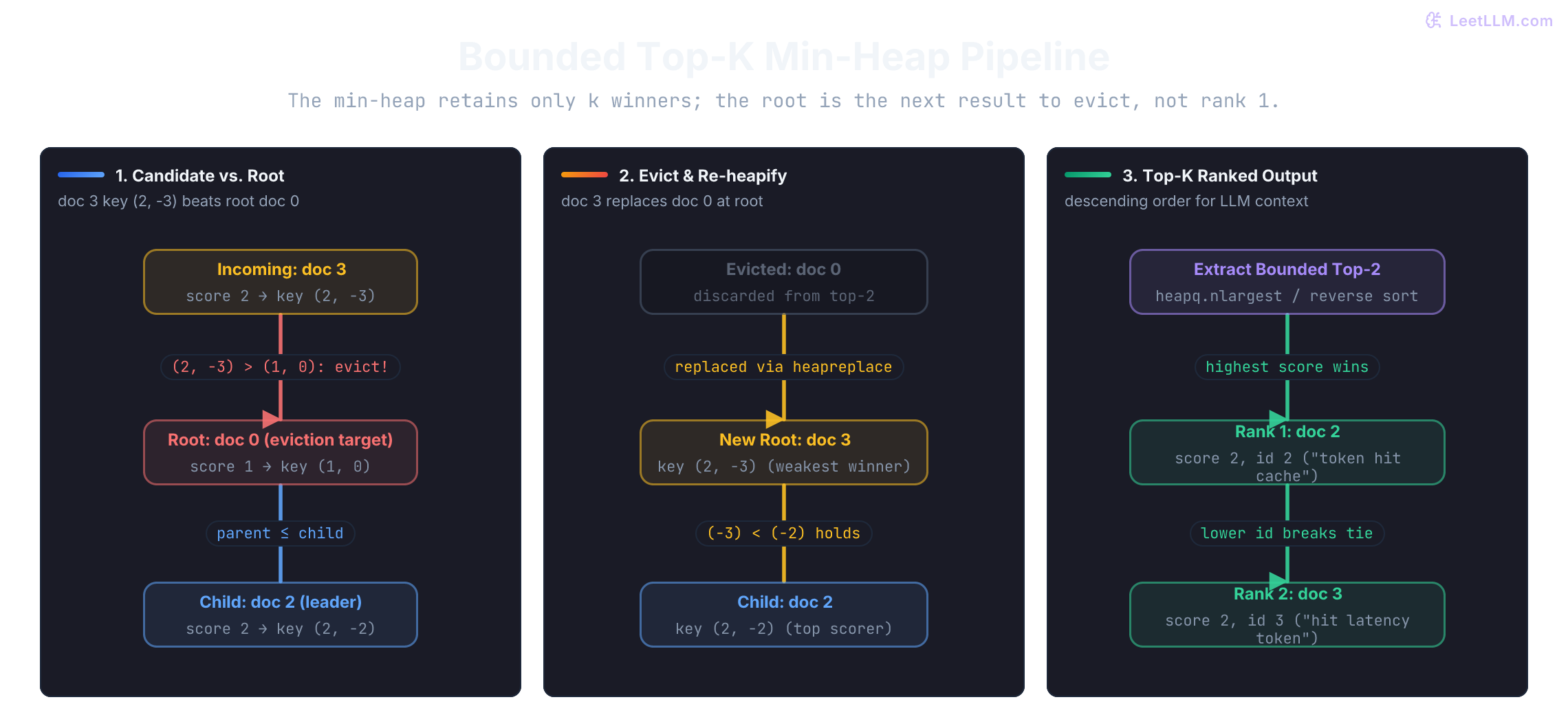
Real rankers need an explicit tie-break rule. The heap demo and retriever lab both prefer the lower document ID when scores tie, which keeps output deterministic.

import heapq

candidate_scores = [(0, 1), (2, 2), (3, 2), (4, 0)]
k = 2
top_k: list[tuple[int, int]] = []

for doc_id, score in candidate_scores:
    # Same key rule as search(): higher score wins; lower doc_id wins ties.
    candidate = (score, -doc_id)
    if len(top_k) < k:
        heapq.heappush(top_k, candidate)
    elif candidate > top_k[0]:
        evicted = heapq.heapreplace(top_k, candidate)
        print("evicted", (evicted[0], -evicted[1]))
    else:
        print("discarded", (score, doc_id))

print("top k", [(score, -doc_key) for score, doc_key in sorted(top_k, reverse=True)])

evicted (1, 0)
discarded (0, 4)
top k [(2, 2), (2, 3)]

The lab later calls heapq.nlargest, which returns results in descending key order. It's suited to selecting a small k from many candidates.^{[5]Reference 5heapq: Heap queue algorithmhttps://docs.python.org/3/library/heapq.html} CPython can use a full sort when k is at least the number of candidates, so the tiny lab isn't a demonstration of a speedup. The explicit heap above shows what bounded selection does.

The candidate > top_k[0] check matters: heapreplace always removes the old root, even when the incoming candidate is weaker. The final candidate, doc 4 with score 0, is discarded. Replacing the root unconditionally would remove a score-2 winner and retain score 0.^{[5]Reference 5heapq: Heap queue algorithmhttps://docs.python.org/3/library/heapq.html}

Building a tiny retriever

Return to the original three notes. First implement the scan, then build an index and accumulate scores from postings. This is the retrieval part of RAG (retrieval-augmented generation): a language model could later read the returned documents. There's no language model in this lab.

Put this in data_structures_demo.py. The tokenizer lowercases and splits on whitespace. Production tokenizers also handle punctuation and language-specific rules, but keeping normalization tiny makes the structure visible. Returning a set means this example scores binary term membership: each distinct query term contributes at most once.

from collections import defaultdict
import heapq

docs = [
    "red bird sings",
    "blue whale swims",
    "red fox sleeps",
]

def tokenize(text: str) -> set[str]:
    return set(text.lower().split())

def slow_search(query: str) -> list[tuple[int, int]]:
    terms = tokenize(query)
    matches: list[tuple[int, int]] = []
    for doc_id, text in enumerate(docs):
        words = tokenize(text)
        score = sum(term in words for term in terms)
        if score:
            matches.append((doc_id, score))
    return matches

def build_index(documents: list[str]) -> dict[str, set[int]]:
    postings: dict[str, set[int]] = defaultdict(set)
    for doc_id, text in enumerate(documents):
        for term in tokenize(text):
            postings[term].add(doc_id)
    return postings

index = build_index(docs)

def search(query: str, k: int = 2) -> list[int]:
    if k < 1 or not query.strip():
        return []

    scores: dict[int, int] = defaultdict(int)
    for term in tokenize(query):
        for doc_id in index.get(term, set()):
            scores[doc_id] += 1

    best = heapq.nlargest(
        k,
        scores.items(),
        key=lambda item: (item[1], -item[0]),
    )
    return [doc_id for doc_id, _score in best]

print("slow scan", slow_search("red fox"))
print("posting list", sorted(index["red"]))
print("search", search("red fox"))

slow scan [(0, 1), (2, 2)]
posting list [0, 2]
search [2, 0]

Read the two outputs as two different contracts. slow_search returns score tuples in corpus order, so (2, 2) appears after (0, 1). Those tuples expose the score trace without ranking it. search uses the posting lists, applies top-k selection, and returns [2, 0].

defaultdict(set) creates an empty set when a missing key is accessed with brackets during indexing. During search, index.get(term, set()) returns an empty set for an unknown term without inserting it into the index. A query for otter therefore returns []. Repeated query words are removed by tokenize, so red red fox scores exactly like red fox.

Map each operation to one structure

The heap key uses score first and negative document ID second. Higher scores win; lower IDs win ties. That small rule makes repeated runs predictable, so a later debugging trace can distinguish a ranking bug from a tie-break choice.

When order and reuse become the problem

The retriever chose structures by lookup and ranking. Ingestion asks a different question: which job arrived first? Repeated queries ask another: can this result be reused without becoming stale?

Process arrivals in order

New documents arrive and wait to be indexed. Later systems may also split them into chunks and encode each chunk as an embedding, a numerical representation used for similarity search. For one class of equal-priority jobs, arrival order is a clean baseline. The operation isn't "find by key" or "keep the best"; it removes the oldest item.

A queue is the behavior: first in, first out (FIFO). Python's collections.deque is the container used here. Its name means double-ended queue, and it supports appends and pops at either end in approximately constant time: more waiting jobs don't require shifting all existing references. Middle indexing becomes slower, so it isn't a replacement for a list when random position access is the main job.^{[6]Reference 6collections: Container datatypeshttps://docs.python.org/3/library/collections.html}

Why does list.pop(0) hurt? A standard Python list stores item references in a single contiguous array. Calling pop(0) removes the head element, which forces CPython to shift every subsequent reference left by one slot. If 50,000 document ingestion jobs or token chunks sit in a queue, draining them item by item incurs quadratic $O(n^2)$ total work.

A FIFO contract doesn't require one particular layout. For example, vLLM's first-come, first-served request queue uses a deque.^{[7]Reference 7vLLM request queue implementationshttps://github.com/vllm-project/vllm/blob/main/vllm/v1/core/sched/request_queue.py} Another implementation is a circular ring buffer: a fixed-size array whose read and write positions advance modulo capacity ((tail + 1) % capacity). Appends and pops update offsets without shifting existing elements. A full buffer still needs a policy: wait, reject the new item, or overwrite an old one.

Which policy would you choose for an embedding job queue? Overwriting can be useful for a recent-token history, but silently dropping the oldest unprocessed document loses work. Python's deque(maxlen=...) discards items from the opposite end when an append fills a bounded deque, so adding maxlen isn't a safe job-queue capacity limit by itself.^{[6]Reference 6collections: Container datatypeshttps://docs.python.org/3/library/collections.html}

Trace the state from left (oldest) to right (newest). Predict the next job after each operation:

from collections import deque

embedding_jobs = deque(["doc-3", "doc-4", "doc-5"])
next_job = embedding_jobs.popleft()

print("next job", next_job)
print("remaining", list(embedding_jobs))

next job doc-3
remaining ['doc-4', 'doc-5']

The rule is simple:

• append new work on one side
• pop the oldest work from the other side

That's FIFO behavior. If you accidentally process newest work first, old jobs can wait indefinitely while new jobs keep arriving. A test should fail when the newest job leaves first.

An in-memory deque shows ordering, not durability. If a worker writes an embedding and crashes before recording completion, a broker may retry the job. The downstream write needs a durable idempotency key so the retry can't create a duplicate vector. The next chapter puts that guarantee in a database transaction and a uniqueness constraint.

The failure case makes the ordering bug visible. New jobs belong at the tail; putting them at the front lets recent uploads jump ahead of old work. Run it before trusting the queue:

from collections import deque

fifo_jobs = deque(["oldest-doc"])
fifo_jobs.extend(["new-doc-a", "new-doc-b"])

newest_first_jobs = deque(["oldest-doc"])
newest_first_jobs.appendleft("new-doc-a")
newest_first_jobs.appendleft("new-doc-b")

print("FIFO runs", fifo_jobs.popleft())
print("wrong order runs", newest_first_jobs.popleft())

FIFO runs oldest-doc
wrong order runs new-doc-b

FIFO also describes claim order, not completion order. Two workers may claim doc 3 and then doc 4, yet doc 4 can finish first. Code that publishes embeddings must bind each result to its document ID rather than assume completion order matches arrival order.

Sharing a container introduces another promise: one worker must claim each item through one synchronized operation. Separate checks and mutations don't become one transaction because a container supports thread-safe individual operations. The following program deliberately interleaves two workers without threads, so the race is reproducible. It also contrasts a history buffer that drops work with a job queue that rejects excess work.^{[6]Reference 6collections: Container datatypeshttps://docs.python.org/3/library/collections.html}

from collections import deque
from queue import Empty, Full, Queue

jobs = deque(["doc-3"])
worker_a_saw_work = bool(jobs)
print("worker B claimed", jobs.popleft())
if worker_a_saw_work:
    try:
        jobs.popleft()
    except IndexError:
        print("worker A's earlier check is stale")

history = deque(["doc-3"], maxlen=1)
history.append("doc-4")
print("bounded deque retained", list(history))

work = Queue(maxsize=1)
work.put_nowait("doc-3")
try:
    work.put_nowait("doc-4")
except Full:
    print("doc-4 rejected; producer must retry or defer it")
print("claimed", work.get_nowait())
try:
    work.get_nowait()
except Empty:
    print("no work available at the moment of claim")

worker B claimed doc-3
worker A's earlier check is stale
bounded deque retained ['doc-4']
doc-4 rejected; producer must retry or defer it
claimed doc-3
no work available at the moment of claim

Queue supplies locking for threads and bounded admission. Use get_nowait() and handle Empty, or wait with get(timeout=...); don't treat an earlier empty() check as a reservation. A rejected producer still owns its unaccepted job. This fixture neither performs embedding work nor acknowledges completion, and the queue remains in memory.^{[8]Reference 8queue: A synchronized queue classhttps://docs.python.org/3/library/queue.html}

Reuse results without serving stale answers

If users ask the same question repeatedly, recomputing retrieval results per request wastes work. A cache can remove that repeated computation, but only if its hit is still valid.

A retrieval cache stores prior ranked document IDs so the system can reuse them. A cache isn't one primitive structure. It combines a mapping from key to value with policies for freshness and eviction. The mapping finds a candidate result; policies decide whether keeping that result stays safe.

cache: dict[tuple[int, str, int], list[int]] = {}
corpus_version = 1
query = "red fox"
k = 2

cache_key = (corpus_version, query, k)
if cache_key not in cache:
    cache[cache_key] = search(query, k)

print("cached", cache[cache_key])

cached [2, 0]

Who owns that list after a cache hit? If the caller removes an inaccessible document from the cached list itself, it changes what the next request sees. Predict the second hit after this attempted per-request filter:

borrowed = cache[cache_key]
borrowed.remove(2)
print("next hit after caller mutation", cache[cache_key])

# Store an immutable sequence; each request owns its own working list.
frozen_cache = {cache_key: tuple(search(query, k))}
request_result = list(frozen_cache[cache_key])
request_result.remove(2)
print("request-local filtered result", request_result)
print("unchanged cached ranking", list(frozen_cache[cache_key]))
cache[cache_key] = search(query, k)  # Restore the earlier teaching fixture.

next hit after caller mutation [0]
request-local filtered result [0]
unchanged cached ranking [2, 0]

This repairs shared mutation, not permission correctness. Filter or scope retrieval before selecting top-k; removing forbidden items afterward can leave too few results or miss accessible winners. The tuple is immutable and contains immutable integers. A tuple containing mutable document objects would still share those objects.^{[3]Reference 3Built-in Typeshttps://docs.python.org/3/library/stdtypes.html}

Make freshness part of the key

If document 2 changes to fox sleeps, its score falls to 1. It now ties with doc 0, so the correct ranking becomes [0, 2], not the cached [2, 0]. Rebuild the affected index and advance corpus_version before serving queries against the new corpus. Changing the version alone can't repair an old index.

Every input that can change the result belongs in the key or in an invalidation rule. Our lab fixes the scoring rule and has no user-specific documents. A shared service must also separate permission scopes and invalidate results when scoring or normalization changes. Two people sending identical text aren't necessarily allowed to retrieve the same notes.

The demo dictionary can grow without limit. A long-running service also needs a bound such as a maximum entry count or byte budget, plus an eviction policy. Least recently used (LRU) discards the entry that hasn't been accessed for the longest time. With two cache slots, the order changes even on a hit:

Versioning prevents stale hits. Eviction bounds storage, even when all entries are still valid. A plain insertion-ordered dictionary doesn't implement LRU by itself: reading a key doesn't move it to the end. OrderedDict.move_to_end() and popitem(last=False) provide the operations needed for this recency order.^{[6]Reference 6collections: Container datatypeshttps://docs.python.org/3/library/collections.html}

Keep k=2 fixed for this failure example. A text-only key finds yesterday's ranking after an update; a versioned key misses and forces recomputation from the updated index.

query = "red fox"
old_version = 1
new_version = 2

text_only_cache = {query: [2, 0]}
versioned_cache = {(old_version, query, 2): [2, 0]}

print("text-only stale hit", query in text_only_cache)
print("versioned stale hit", (new_version, query, 2) in versioned_cache)

updated_docs = docs.copy()
updated_docs[2] = "fox sleeps"
original_index = index
print("new version with old index", search(query))
index = build_index(updated_docs)
print("rebuilt index ranking", search(query))
assert search(query) == [0, 2]
index = original_index  # Keep later exercises on the original corpus.

text-only stale hit True
versioned stale hit False
new version with old index [2, 0]
rebuilt index ranking [0, 2]

The miss only triggers a computation; it doesn't establish that computation used current postings. In a shared service, build a replacement corpus/index snapshot, then publish it together with its version under the service's synchronization rule. Each query must use one matching snapshot and version throughout. Updating the version first and the index later exposes a window where a stale ranking can be stored under the new key.

Use paths, links, and prefixes

Lists, dictionaries, sets, deques, and heaps covered position, identity, arrival order, and priority. What if the query asks for a path instead? Three other shapes become useful when the question is about hierarchy, a relationship, or a shared prefix.^{[1]Reference 1Introduction to Algorithms (3rd ed.)https://mitpress.mit.edu/9780262033848/introduction-to-algorithms/}

A tree gives each node one parent path

A rooted tree has a chosen root, parent-child edges, and no cycles. Every node except the root has exactly one parent. In a topic taxonomy, each note follows one path from the root:

notes
├── red animals
│   ├── doc 0: red bird sings
│   └── doc 2: red fox sleeps
└── blue animals
    └── doc 1: blue whale swims

That shape makes subtree questions natural: "show every note under red animals." A binary search tree solves a different problem: it orders keys so smaller keys lie in a node's left subtree and larger keys in its right subtree. Each comparison chooses a branch. A balanced tree needs only a logarithmic number of such choices; a badly skewed tree becomes a chain. A topic hierarchy isn't automatically a search tree.

A heap is also drawn as a tree, but it isn't a binary search tree. A min-heap guarantees only that each parent is no larger than its children. It doesn't support arbitrary key search the way a search tree does. Its job is still priority eviction.

A graph allows many-to-many links

Suppose doc 2 belongs under both red animals and foxes, or doc 0 links directly to doc 2. One-parent taxonomy no longer captures the relationship cleanly. A graph stores vertices (nodes) and edges (links); edges may be directed or undirected, and graphs may contain cycles. Choose it when the links themselves are the data you need to traverse.

Python code commonly represents a sparse graph as a dictionary of neighbor sets:

from collections import deque

links = {
    0: {2},
    1: set(),
    2: {0},
}

print("neighbors of doc 0", sorted(links[0]))
pending = deque([0])
discovered = {0}
visit_order = []
while pending:
    doc_id = pending.popleft()
    visit_order.append(doc_id)
    for neighbor in sorted(links.get(doc_id, set())):
        if neighbor not in discovered:
            discovered.add(neighbor)  # Mark when queued, not after expansion.
            pending.append(neighbor)
print("reachable from doc 0", visit_order)

neighbors of doc 0 [2]
reachable from doc 0 [0, 2]

The first printout [2] exposes one edge. The second shows a bounded traversal: doc 2's reverse link reaches doc 0, but doc 0 is already discovered and isn't queued again. Marking a node when it's queued also prevents several parents from adding duplicate pending work before that node is processed. With a fixed graph, each reachable node enters this queue once.

If a traversal can encounter 0 -> 2 -> 0, it needs a visited set. Without one, the search can loop forever. Graph cost depends on representation: an adjacency list stores outgoing neighbors compactly for sparse links, while a matrix makes every possible pair explicit. Representation follows the density and operation of the links.

A trie follows one symbol per edge

A trie, also called a prefix tree, organizes strings by shared prefixes. If the product asks "what completions start with fo?", shared characters should be traversed once. Allowed terms fox, food, and fog share the path f -> o, then branch:

(root)
└── f
    └── o
        ├── x              fox [end]
        ├── o -> d         food [end]
        └── g              fog [end]

Looking up prefix fo follows two edges from the empty root before enumerating matching suffixes. An end marker distinguishes a complete term from a prefix: if fox were also a prefix of a longer allowed term, its node would still need an end marker even though it had children. Reaching the prefix depends on prefix length, not on how many unrelated words exist. Returning completions still costs time to traverse and produce those matches. Tries can use substantial memory for nodes and child links, so compressed variants merge unbranched paths.

Prefix trees answer "what strings start with this prefix?" Graphs model dependencies and knowledge links. Trees model module, configuration, and taxonomy hierarchies. The shape still follows the operation, even when several shapes can represent the same records.

Compare the work each operation does

Big-O describes how an upper bound on work grows with input size. O(1) stays bounded as the collection grows; O(n) grows linearly. O(log n) grows slowly: doubling the input adds only a constant number of steps for a balanced-tree lookup. These labels don't predict wall-clock time. The later complexity lesson develops the notation more carefully.

In this table, n is items in a structure, m is scored candidates, k is retained winners, V is graph vertices, E is graph edges, and p is prefix length. The bounds assume bounded-cost key comparisons and hashes; reading a long string key has its own cost.^{[1]Reference 1Introduction to Algorithms (3rd ed.)https://mitpress.mit.edu/9780262033848/introduction-to-algorithms/}

Use the table to compare operations, not to crown one structure fastest. A list index is cheap when the position is known. A list scan is cheap to write but grows with every item. The right row depends on the question that dominates your workload.

The retriever has more than one cost. Expected dictionary lookup reaches each posting set quickly, but it still scans returned postings. A common term may appear in almost every document. If m candidates receive scores, bounded selection adds O(m log k) work for 2 <= k <= m. The scores dictionary also holds up to m entries, so the lab's total query memory includes those scores as well as the heap's O(k) storage. Constant-time key lookup never makes the whole query constant-time.

Diagnose the wrong shape

The first working loop often feels good enough, so it stays even after it becomes slow, duplicated, stale, or impossible to finish. Diagnose the operation before choosing a structure:

The fastest way to debug is still the same: trace one tiny example by hand. Make the operation and its promise visible before changing the container.

Check the structures when the ranking looks right

The final ranking can look right while an intermediate promise is broken. These tests check the structures as well as the result:

from collections import deque

def test_red_lookup_has_two_docs():
    assert index["red"] == {0, 2}

def test_empty_query_returns_empty_list():
    assert search("") == []

def test_indexed_search_matches_ranked_scan():
    for query in ["red fox", "red", "Red FOX", "red red fox", "otter", ""]:
        ranked = sorted(slow_search(query), key=lambda item: (-item[1], item[0]))
        for k in [0, 1, 2, 5]:
            assert search(query, k) == [doc_id for doc_id, _score in ranked[:k]]

def test_search_normalizes_case():
    assert search("Red FOX") == [2, 0]

def test_queue_is_fifo():
    jobs = deque(["doc-3", "doc-4"])
    assert jobs.popleft() == "doc-3"

def test_graph_cycle_is_bounded_by_visited_set():
    links = {0: {2}, 2: {0}}
    visited: set[int] = {0}
    pending = deque([0])
    while pending:
        doc_id = pending.popleft()
        for neighbor in links.get(doc_id, set()):
            if neighbor not in visited:
                visited.add(neighbor)
                pending.append(neighbor)
    assert visited == {0, 2}

test_red_lookup_has_two_docs()
test_empty_query_returns_empty_list()
test_indexed_search_matches_ranked_scan()
test_search_normalizes_case()
test_queue_is_fifo()
test_graph_cycle_is_bounded_by_visited_set()
print("six structural tests passed")

six structural tests passed

Each test checks one promise:

• the index maps terms to the right documents
• empty input is predictable
• indexed ranking matches the scan, including ties, unknown terms, repeated terms, and different result limits
• query normalization is consistent
• queue order stays first-in, first-out
• graph traversal terminates across a cycle

Predict the next operation on paper

Pause before looking at the solution sketches. Predict the next operation, then name the structure that makes it cheap or safe:

1. Add a fourth document with docs.append("red fox runs"), then rebuild with index = build_index(docs).
2. Predict sorted(index["red"]).
3. Predict search("red fox").
4. Run search("otter") and explain why it shouldn't crash.
5. Change document 2 so it no longer contains red, then explain what must happen to the cache.
6. Choose a structure for each new requirement: autocomplete the prefix fo; represent notes with several cross-links; process oldest upload first.
7. Explain why a min-heap isn't a sorted list and why a heap isn't a binary search tree.

Solution sketches

Use these to check your reasoning, not to skip the exercise.

If an answer is hard to check, go back to the score table. Predict the work each operation forces before the code hides it.

Hand the promises to durable storage

The inverted index, deque, and versioned cache you built live in one process. Close the process and they're gone. Share them across two workers and you also need identity, uniqueness, and freshness that survive a restart.

A list is for position, a hash map for identity, a deque for oldest work, a heap for the weakest retained result, and a trie for a prefix. Those promises are still local to one process. Two processes that must return the same lookup after a restart need those promises stored where the restart cannot erase them.