Personalize this lesson
Adapt explanations and teaching visuals to your background and preferred voice.
A training run reports steadily dropping loss, yet its saved incident router behaves erratically the moment you deploy it to staging. Nothing threw an exception. No crash log appeared in your terminal. Behind that quiet execution, one of several silent state bugs occurred: gradients carried over between mini-batches, Dropout stayed active during validation, or saving a live reference meant subsequent epochs quietly mutated your supposedly frozen checkpoint. We'll build an automated ticket router from scratch and trace every one of these state transitions directly.
Suppose an upstream NLP feature pipeline converts each incoming customer ticket into two normalized numerical features: an urgency score and a severity-language score. A binary target indicates whether the ticket requires specialist escalation (1) or standard routing (0). Untrained linear weights guess no better than a coin flip. A training loop passes examples forward through the model, measures prediction error with a loss function, calculates how each individual weight contributed to that error, and updates the weights in the direction of steepest descent.
The earlier causal reasoning lesson explains how to test whether a deployed model update actually improves user outcomes. An A/B test provides that evaluation. Neither technique builds the model itself. First, the loop has to learn it.
PyTorch doesn't hide this learning cycle behind a monolithic .fit() call: you write the loop yourself. That imperative design makes every tensor, gradient, and memory buffer inspectable at runtime. Later, when you scale up to fine-tune a large language model or run distributed training across multiple nodes, the fundamental handoffs remain identical: batches, logits, loss, gradients, optimizer updates, validation passes, and durable checkpoints.[1][2]
The gradient descent and cross-entropy concepts build on backpropagation and softmax classification. Here we implement them in executable PyTorch code. Each code example runs self-contained on CPU unless explicitly noted otherwise. The small numbers are designed to expose tensor mechanics clearly rather than optimize classification accuracy.
These examples were validated on PyTorch 2.x on CPU. Random seeds make the fixtures repeatable, but floating-point numbers can vary across different architectures or CUDA backends. Check the stated invariants, such as monotonic loss reduction or matching reloaded logits, rather than treating a last-decimal discrepancy as an error.[3]
Turn a ticket into tensors
We'll bypass raw text tokenization for now. The feature extraction pipeline has converted each incident ticket into two normalized floating-point numbers:
| Feature | Meaning | Example range |
|---|---|---|
urgency | Phrases signaling strict deadlines, financial loss, or security exposure | -2.0 to 2.0 |
severity_language | Words indicating system outages, downtime, or broad customer impact | -2.0 to 2.0 |
label | 0 = standard queue, 1 = specialist escalation | 0 or 1 |
Every training instance consists of a two-element feature vector and an integer class target. A mini-batch stacks those rows into a two-dimensional tensor. Six incident tickets produce a feature tensor of shape (6, 2) and a label tensor of shape (6,).
1import torch
2
3features = torch.tensor(
4    [
5        [-2.0, -1.2],
6        [-1.3, -0.8],
7        [-0.8, -1.4],
8        [0.9, 1.1],
9        [1.4, 0.8],
10        [1.8, 1.6],
11    ],
12    dtype=torch.float32,
13)
14labels = torch.tensor([0, 0, 0, 1, 1, 1], dtype=torch.long)
15
16print("features:", tuple(features.shape), features.dtype)
17print("labels:", tuple(labels.shape), labels.dtype)
18print("first ticket:", features[0].tolist(), "route:", labels[0].item())1features: (6, 2) torch.float32
2labels: (6,) torch.int64
3first ticket: [-2.0, -1.2000000476837158] route: 0That output represents a strict interface contract. Floating-point features (torch.float32) pass through linear matrix multiplications, while integer targets (torch.long, equivalent to 64-bit integers) supply class indices. Mismatched shapes or floating targets will cause downstream loss functions to fail immediately.
Now that inputs and targets match the expected shapes, inspect how the model scores each ticket before introducing optimization.
Logits are scores, not probabilities
A linear classification head ending in nn.Linear(2, 2) produces two unconstrained scores for each ticket:
| Output column | Destination route |
|---|---|
0 | standard queue |
1 | specialist escalation |
These unnormalized outputs are logits. Logits can be positive, negative, or zero, and their values don't sum to one. For multi-class classification, PyTorch's nn.CrossEntropyLoss expects these raw logits alongside integer target indices. Under the hood, it combines log-softmax with negative log-likelihood in a single, numerically stabilized operation.[4]
Consider raw ticket logits [2.0, -1.0] for an example whose ground-truth class is 0. To see how cross-entropy scores this prediction, convert the logits to probabilities:
The second ticket outputs logits [-0.5, 1.5] with ground-truth class 1. The correct class wins, but with less margin: , yielding loss . The average loss over both tickets is . PyTorch's default reduction="mean" computes exactly this batch average.
1import torch
2from torch import nn
3
4logits = torch.tensor([[2.0, -1.0], [-0.5, 1.5]], dtype=torch.float32)
5labels = torch.tensor([0, 1], dtype=torch.long)
6loss = nn.CrossEntropyLoss()(logits, labels)
7
8routes = ["standard", "escalate"]
9predictions = logits.argmax(dim=1).tolist()
10print("predicted routes:", [routes[index] for index in predictions])
11print("cross entropy:", round(loss.item(), 4))1predicted routes: ['standard', 'escalate']
2cross entropy: 0.0878Failure case: Don't pass
torch.softmax(logits, dim=-1)intoCrossEntropyLoss. The loss function expects unnormalized logits. If you pass probabilities,CrossEntropyLosstreats them as raw scores and applies a second softmax normalization, distorting the objective and corrupting gradient calculations. A naive manual calculation liketorch.log(torch.softmax(logits))can also overflow or underflow when logits are large or small, whereasCrossEntropyLossuses the log-sum-exp trick internally: , where .
Why should CrossEntropyLoss receive raw logits rather than probabilities from a separate softmax?
Answer
It combines log-softmax and negative log-likelihood in a numerically stable operation using the log-sum-exp trick. Applying softmax first makes the loss treat probabilities as unnormalized scores and apply another normalization, altering the objective and its gradients.
CrossEntropyLoss summarizes batch predictions into a single scalar value. That scalar quantifies the model's current error, but it hasn't changed any weights. To update parameters, we need to trace one batch through the training loop's five execution phases.
The five execution phases in a training step
Every iteration in a PyTorch training step executes five distinct phases in a precise order. Before checking the table below, determine which specific step actually alters the model's weight tensors:
| Phase | PyTorch statement | Purpose | Parameter values change? |
|---|---|---|---|
| 1 | optimizer.zero_grad(set_to_none=True) | Clear stored gradients left by earlier iterations. | No |
| 2 | logits = model(xb) | Run the forward pass and build the autograd computation graph. | No |
| 3 | loss = loss_fn(logits, yb) | Score predictions against ground-truth labels. | No |
| 4 | loss.backward() | Traverse the graph backward to populate .grad attributes. | No |
| 5 | optimizer.step() | Update parameter values using the stored gradients. | Yes |
Calling loss.backward() doesn't modify weight values. It traverses the dynamic computation graph in reverse via the chain rule, computing partial derivatives of the scalar loss with respect to every trainable leaf tensor (requires_grad=True), and stores those values in each parameter's .grad field.[5][6]
The parameter values themselves remain completely unchanged until optimizer.step() runs. The optimizer reads the accumulated gradients, applies its update rule (such as SGD or Adam), and updates the parameter storage in place.
Why use set_to_none=True in optimizer.zero_grad()? Setting .grad = None rather than filling tensors with zeros provides three practical advantages:
- Memory efficiency: Setting
.grad = Noneimmediately deallocates the gradient tensor memory, lowering peak memory consumption between iterations. - Autograd efficiency: When a parameter's
.gradisNone, the autograd engine duringbackward()simply assigns the newly computed gradient tensor (p.grad = grad) instead of performing an in-place addition (p.grad.add_(grad)), saving memory bandwidth and kernel overhead.[7] - Unused parameter behavior: In architectures with conditional routing (such as mixture of experts), parameters not used in a forward pass keep
.grad = None. Optimizers like Adam skip parameters withNonegradients, whereas a zero-filled tensor would cause Adam's weight decay and momentum buffers to update those parameters anyway.
Trace this step with exact arithmetic. Consider two symmetric tickets: ticket [1.0, 1.0] has label 1 (escalate), and ticket [-1.0, -1.0] has label 0 (standard). Let be a 2x2 weight matrix where row 0 scores class 0 and row 1 scores class 1. Initializing with zero bias yields logits [0.0, 0.0] for both tickets. The predicted class probabilities are [0.5, 0.5], producing a cross-entropy loss of for each row.
For cross-entropy loss with mean reduction, each row's gradient contribution to weight is , where is the batch size. Both tickets produce positive gradient values for class 0 weights and negative gradient values for class 1 weights, yielding an aggregate gradient matrix . The bias gradients cancel to zero. loss.backward() leaves at zero while writing into . Finally, SGD with learning rate updates the weights:
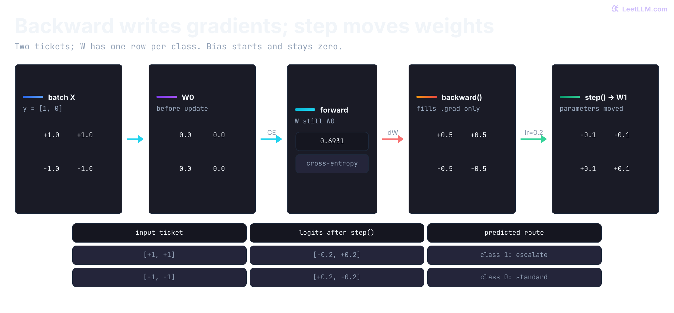
backward() fills dW but leaves W unchanged. With learning rate 0.2, optimizer.step() creates weights [[-0.1, -0.1], [0.1, 0.1]], which route the positive ticket to escalation and the negative ticket to the standard queue.Let's execute this exact mathematical calculation in PyTorch to confirm every state transition.
1import torch
2from torch import nn
3
4features = torch.tensor([[1.0, 1.0], [-1.0, -1.0]], dtype=torch.float32)
5labels = torch.tensor([1, 0], dtype=torch.long)
6model = nn.Linear(2, 2)
7with torch.no_grad():
8    model.weight.zero_()
9    model.bias.zero_()
10
11optimizer = torch.optim.SGD(model.parameters(), lr=0.2)
12loss_fn = nn.CrossEntropyLoss()
13
14before = model.weight.detach().clone()
15optimizer.zero_grad(set_to_none=True)
16loss = loss_fn(model(features), labels)
17loss.backward()
18gradient = model.weight.grad.detach().clone()
19after_backward = model.weight.detach().clone()
20optimizer.step()
21after_step = model.weight.detach().clone()
22
23print("loss:", round(loss.item(), 4))
24print("gradient filled:", bool(gradient.abs().sum() > 0))
25print("changed by backward:", not torch.equal(before, after_backward))
26print("changed by step:", not torch.equal(before, after_step))
27torch.testing.assert_close(gradient, torch.tensor([[0.5, 0.5], [-0.5, -0.5]]))
28torch.testing.assert_close(after_step, torch.tensor([[-0.1, -0.1], [0.1, 0.1]]))1loss: 0.6931
2gradient filled: True
3changed by backward: False
4changed by step: TrueThe output confirms the state boundaries: loss.backward() populated .grad without touching parameter values, and optimizer.step() moved the parameters. What happens if leftover gradients from an earlier iteration remain in .grad when the next backward() executes?
Clearing gradients and micro-batch accumulation
PyTorch adds newly computed gradients into existing .grad buffers rather than overwriting them (param.grad += new_grad). That accumulation default is intentional: it enables gradient accumulation, letting multiple micro-batches build up an effective batch update when memory is constrained. In standard training where each mini-batch should trigger an independent step, failing to clear gradients causes stale derivatives to pollute future updates.
To observe this accumulation directly, differentiate twice at . The derivative is . Calling backward() a second time without clearing gradients adds another , producing an accumulated gradient of . Resetting weight.grad = None restores the clean single-step value:
1import torch
2
3weight = torch.tensor(1.0, requires_grad=True)
4
5(weight**2).backward()
6first_grad = weight.grad.item()
7
8(weight**2).backward()
9accumulated_grad = weight.grad.item()
10
11weight.grad = None
12(weight**2).backward()
13cleared_grad = weight.grad.item()
14
15print("first backward:", first_grad)
16print("without clearing:", accumulated_grad)
17print("after clearing:", cleared_grad)1first backward: 2.0
2without clearing: 4.0
3after clearing: 2.0Without clearing, the derivative silently doubles. Calling optimizer.zero_grad(set_to_none=True) inside the batch loop ensures each update depends solely on its own data.[7]
Gradient accumulation across micro-batches
When a model or batch size exceeds available GPU memory, gradient accumulation lets you simulate a larger effective batch size using smaller micro-batches of size .
The loss function usually averages errors over the current micro-batch: . The true mean loss over the combined batch of examples is:
Because autograd sums gradients across multiple backward() calls, you must divide each micro-batch loss by before backpropagating: (loss / K).backward(). If you skip this division, the accumulated gradient will be times larger than the true average, which acts like multiplying your learning rate by and frequently causes training to diverge.[8]
In distributed training using DistributedDataParallel (DDP), every backward() call triggers an AllReduce network synchronization across all GPUs. Calling AllReduce on every micro-batch wastes network bandwidth. PyTorch provides the model.no_sync() context manager to suppress gradient communication during the first micro-batches, synchronizing gradients across nodes only on the final step right before optimizer.step().[9]
What happens if optimizer.zero_grad() runs only once per epoch instead of once per mini-batch in standard training?
Answer
Each backward pass adds newly computed derivatives into existing .grad buffers. Later updates combine current gradients with stale gradients from earlier batches, destabilizing optimization. Reset inside the batch loop unless accumulation is deliberate.
One update on a synthetic fixture verifies autograd mechanics, but it doesn't constitute a complete loop. We need abstractions to manage datasets and partition rows into mini-batches.
Batching and row-weighted epoch loss
A dataset stores samples and their corresponding labels. A data loader coordinates batching, worker multiprocessing, and shuffling between epochs. Shuffling ensures the optimizer encounters diverse gradient directions across iterations, preventing cyclical oscillation.
Using our six tickets with batch_size=4, the data loader yields two batches: the first contains four rows, and the second contains the remaining two rows.
1import torch
2from torch.utils.data import DataLoader, TensorDataset
3
4features = torch.tensor(
5    [
6        [-2.0, -1.2],
7        [-1.3, -0.8],
8        [-0.8, -1.4],
9        [0.9, 1.1],
10        [1.4, 0.8],
11        [1.8, 1.6],
12    ],
13    dtype=torch.float32,
14)
15labels = torch.tensor([0, 0, 0, 1, 1, 1], dtype=torch.long)
16loader = DataLoader(TensorDataset(features, labels), batch_size=4, shuffle=False)
17
18for batch_index, (xb, yb) in enumerate(loader, start=1):
19 print(f"batch {batch_index}: shape={tuple(xb.shape)} labels={yb.tolist()}")1batch 1: shape=(4, 2) labels=[0, 0, 0, 1]
2batch 2: shape=(2, 2) labels=[1, 1]The final batch contains only two rows. When calculating average loss across an epoch, don't simply average the reported batch loss numbers. Because batch sizes differ, taking an unweighted mean of batch averages assigns excessive influence to the smaller batch.
To compute the exact epoch loss, weight each batch mean by its row count: sum the batch losses multiplied by their batch sizes, then divide by the total number of rows across the entire dataset. For instance, batches of size 4 and 2 with average losses 0.20 and 0.50 yield a true epoch average of , whereas an unweighted average of the two numbers would report .[4]
With data loading established, we can construct a minimal training loop. Before evaluating generalization on held-out data, we test whether the model can memorize a small, clean batch.
Overfitting one batch as an isolation test
Before training on large datasets, run an overfit-one-batch test. Take a single batch of clean, separable examples and verify that the model drives training loss to near zero. If the model can't memorize eight clean rows, don't debug data distributions or regularization: inspect label encodings, tensor shapes, loss configurations, learning rate scale, and the order of optimizer operations.
We'll define a multi-layer classifier: nn.Linear(2, 8) expands the two inputs to eight hidden activations, nn.ReLU() introduces non-linearity by zeroing negative values, and nn.Linear(8, 2) produces class logits.
1import torch
2from torch import nn
3
4torch.manual_seed(7)
5features = torch.tensor(
6    [
7        [-2.0, -1.2], [-1.3, -0.8], [-0.8, -1.4], [-1.6, -0.4],
8        [0.9, 1.1], [1.4, 0.8], [1.8, 1.6], [0.7, 1.7],
9    ],
10    dtype=torch.float32,
11)
12labels = torch.tensor([0, 0, 0, 0, 1, 1, 1, 1], dtype=torch.long)
13model = nn.Sequential(nn.Linear(2, 8), nn.ReLU(), nn.Linear(8, 2))
14loss_fn = nn.CrossEntropyLoss()
15optimizer = torch.optim.SGD(model.parameters(), lr=0.15)
16
17with torch.no_grad():
18    initial_loss = loss_fn(model(features), labels).item()
19
20for _ in range(120):
21    optimizer.zero_grad(set_to_none=True)
22    loss = loss_fn(model(features), labels)
23    loss.backward()
24    optimizer.step()
25
26with torch.no_grad():
27    final_logits = model(features)
28    final_loss = loss_fn(final_logits, labels).item()
29    accuracy = (final_logits.argmax(dim=1) == labels).float().mean().item()
30
31print("initial loss:", round(initial_loss, 4))
32print("final loss:", round(final_loss, 4))
33print("memorized batch:", accuracy == 1.0)1initial loss: 0.6521
2final loss: 0.0056
3memorized batch: TrueThe loss drops from 0.6521 to 0.0056 and classification accuracy reaches 100%. This passes the basic wiring check. Now we can separate training from held-out validation.
Isolating validation from training updates
Memorizing training rows proves that gradients flow through the model, but it provides zero evidence that the classifier generalizes to unseen tickets. To assess generalization, split the workflow into two phases:
- Training phase: Mini-batches flow forward, autograd constructs the computation graph,
loss.backward()calculates derivatives, andoptimizer.step()updates parameters. - Validation phase: Held-out examples evaluate the current weights without updating parameters or recording gradient history.
Validation relies on two independent controls:
| Control | Responsibility |
|---|---|
model.eval() | Configures layers like Dropout and batch normalization (BatchNorm) for evaluation. |
torch.no_grad() | Halts autograd graph construction, saving compute and memory. |
The script below trains on eight tickets and tracks validation loss across four held-out tickets over 60 epochs.
1import copy
2import torch
3from torch import nn
4from torch.utils.data import DataLoader, TensorDataset
5
6torch.manual_seed(7)
7train_x = torch.tensor(
8    [
9        [-2.0, -1.2], [-1.3, -0.8], [-0.8, -1.4], [-1.6, -0.4],
10        [0.9, 1.1], [1.4, 0.8], [1.8, 1.6], [0.7, 1.7],
11    ],
12    dtype=torch.float32,
13)
14train_y = torch.tensor([0, 0, 0, 0, 1, 1, 1, 1], dtype=torch.long)
15val_x = torch.tensor([[-1.1, -0.6], [-0.5, -1.7], [1.0, 0.6], [1.7, 0.4]])
16val_y = torch.tensor([0, 0, 1, 1], dtype=torch.long)
17
18loader = DataLoader(TensorDataset(train_x, train_y), batch_size=4, shuffle=True)
19model = nn.Sequential(nn.Linear(2, 8), nn.ReLU(), nn.Linear(8, 2))
20loss_fn = nn.CrossEntropyLoss()
21optimizer = torch.optim.SGD(model.parameters(), lr=0.15)
22best_loss = float("inf")
23best_state = None
24best_epoch = None
25
26for epoch in range(1, 61):
27    model.train()
28    train_total = 0.0
29    train_count = 0
30    for xb, yb in loader:
31        optimizer.zero_grad(set_to_none=True)
32        loss = loss_fn(model(xb), yb)
33        if not torch.isfinite(loss):
34            raise RuntimeError(f"non-finite training loss at epoch {epoch}")
35        loss.backward()
36        optimizer.step()
37        train_total += loss.item() * len(yb)
38        train_count += len(yb)
39
40    model.eval()
41    with torch.no_grad():
42        val_logits = model(val_x)
43        val_loss = loss_fn(val_logits, val_y).item()
44    if not torch.isfinite(torch.tensor(val_loss)):
45        raise RuntimeError(f"non-finite validation loss at epoch {epoch}")
46
47    if val_loss < best_loss:
48        best_loss = val_loss
49        best_epoch = epoch
50        best_state = copy.deepcopy(model.state_dict())
51
52assert best_state is not None
53model.load_state_dict(best_state)
54model.eval()
55with torch.no_grad():
56    selected_accuracy = (model(val_x).argmax(dim=1) == val_y).float().mean().item()
57
58print("best validation loss:", round(best_loss, 4))
59print("selected epoch:", best_epoch)
60print("selected validation accuracy:", round(selected_accuracy, 3))
61print("saved tensors:", len(best_state))1best validation loss: 0.0118
2selected epoch: 60
3selected validation accuracy: 1.0
4saved tensors: 4The checkpoint snapshot aliasing trap
Notice the call to copy.deepcopy(model.state_dict()) in line 432 above. A common bug is writing best_state = model.state_dict(). Calling model.state_dict() returns a dictionary containing direct references to the live parameter tensors. As future epochs update model weights, those changes mutate the referenced tensors. Your saved best_state quietly drifts toward the final epoch's weights rather than preserving the best checkpoint.[10]
We can demonstrate this reference leak directly:
1import copy
2import torch
3from torch import nn
4
5model = nn.Linear(2, 2)
6with torch.no_grad():
7    model.weight.zero_()
8
9aliased = model.state_dict()
10snapshot = copy.deepcopy(model.state_dict())
11with torch.no_grad():
12    model.weight.add_(1.0)
13
14print("plain state followed the update:", torch.equal(aliased["weight"], model.weight))
15print("copied state stayed at zero:", torch.count_nonzero(snapshot["weight"]).item() == 0)1plain state followed the update: True
2copied state stayed at zero: True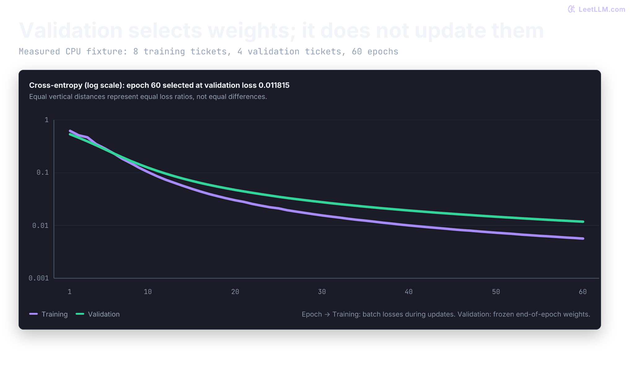
0.535825 at epoch 1 to 0.011815 at epoch 60, which becomes the selected checkpoint with held-out accuracy 1.0. Validation uses eval() and no_grad(); it never calls backward() or step().The validation loop called model.eval() even though the model lacked Dropout or BatchNorm layers. Adding a mode-sensitive layer makes the purpose of that call immediately visible.
Operational modes and context managers
In a network composed strictly of linear transformations and ReLU activations, model.train() and model.eval() yield identical outputs because neither layer maintains mode-dependent state. In production architectures, however, several layers change their behavior across modes:
- Dropout: During training (
train()), Dropout randomly zeroes activations with probability and scales surviving activations by to preserve expected magnitude. During evaluation (eval()), Dropout acts as an identity pass-through. - BatchNorm: During training, BatchNorm computes mean and variance across the current mini-batch and updates its exponential moving average running buffers (
running_mean,running_var). During evaluation, it freezes buffer updates and normalizes activations using the accumulated running statistics. - LayerNorm: Unlike BatchNorm, LayerNorm normalizes across the hidden channel dimensions of each sample independently. Its forward pass is identical in both
train()andeval().
The snippet below introduces Dropout to our classifier, runs the same input ticket twice in training mode, and then runs it twice in evaluation mode.
1import torch
2from torch import nn
3
4torch.manual_seed(0)
5model = nn.Sequential(nn.Linear(2, 6), nn.ReLU(), nn.Dropout(p=0.5), nn.Linear(6, 2))
6ticket = torch.tensor([[1.2, 0.9]])
7
8model.train()
9train_a = model(ticket)
10train_b = model(ticket)
11
12model.eval()
13with torch.no_grad():
14    eval_a = model(ticket)
15    eval_b = model(ticket)
16
17print("training outputs equal:", torch.equal(train_a, train_b))
18print("evaluation outputs equal:", torch.equal(eval_a, eval_b))1training outputs equal: False
2evaluation outputs equal: TrueThe output illustrates the separation of responsibilities: model.eval() controls layer-specific operational logic, while torch.no_grad() controls autograd tape construction. Calling one without the other addresses only half of validation.
Why do validation loops require both model.eval() and torch.no_grad()?
Answer
model.eval() switches mode-sensitive layers (like Dropout and BatchNorm) into deterministic evaluation behavior. torch.no_grad() separately stops the autograd engine from constructing a computation graph. Neither replaces the other.
Saving weights to disk produces the deployable artifact. Checkpoints also protect ongoing training against sudden hardware faults and preemption.
Resilient checkpointing and atomic state snapshots
A trained model isn't production-ready until its parameters and configurations are saved in a durable, reloadable format. Never save the Python model instance directly using torch.save(model, path). That approach uses Python's pickle to serialize class definitions and file paths, binding the checkpoint to your exact codebase structure.
Save the model's state dictionary (state_dict) instead. A state_dict is an ordered Python dictionary mapping parameter and buffer names to their underlying tensor storage.
The complete resumption bundle
If training will resume later, saving only model weights is insufficient. A complete checkpoint must capture all state required for exact continuation:
model_state_dict: Trainable parameters and persistent buffers (such as BatchNorm running stats).optimizer_state_dict: Optimization state, including Adam's first moment () and second moment () vectors alongside step counts. If you omit optimizer state upon resumption, momentum resets to zero, causing abrupt parameter oscillations that degrade convergence.[10]lr_scheduler_state_dict: Current learning rate step counter and cycle phase.scaler_state_dict: The dynamic loss scale factor and consecutive finite step count when using Automatic Mixed Precision.rng_state: Random number generator states across PyTorch CPU, CUDA (torch.cuda.get_rng_state_all()), Pythonrandom, and NumPy to ensure exact data shuffling and dropout repeatability upon resumption.[3]- Metadata: The epoch index, global step count, validation metrics, git commit hash, and dataset split identifier.
Preventing corruption with atomic file writes
On compute clusters with spot instances or preemptible cloud nodes, a training process can be terminated without warning. If preemption strikes while torch.save(checkpoint, "checkpoint.pt") is mid-write, the target file is left truncated. When the job restarts, torch.load crashes with EOFError: Ran out of input, permanently destroying days of training progress.
To make checkpointing resilient against preemption, write atomically:
- Serialize the state bundle to a temporary staging file in the same filesystem directory (
checkpoint.pt.tmp). - Flush application buffers and invoke
os.fsync(file_descriptor)to guarantee the operating system commits write caches to physical storage. - Call
os.replace("checkpoint.pt.tmp", "checkpoint.pt"). On POSIX systems,os.replaceis an atomic filesystem operation. At any instant, the filesystem points either to the previous valid checkpoint or the new complete checkpoint, eliminating the risk of corrupted files.
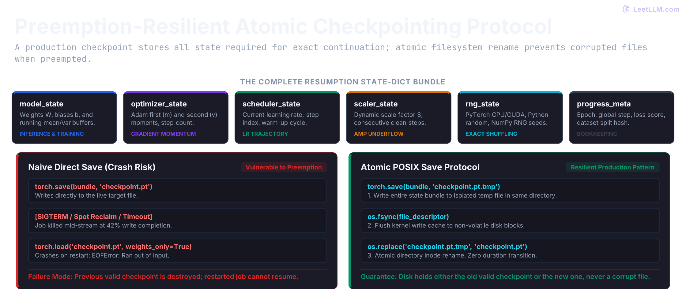
os.fsync followed by atomic os.replace ensures a crash never corrupts on-disk checkpoints.In PyTorch 2.6 and later, torch.load(..., weights_only=True) is the default standard, restricting unpickling to tensors, primitive values, and basic containers to prevent arbitrary code execution vulnerabilities.[11]
1import os
2from pathlib import Path
3from tempfile import TemporaryDirectory
4
5import torch
6from torch import nn
7
8torch.manual_seed(11)
9features = torch.tensor([[-1.5, -1.0], [-0.9, -1.2], [1.1, 0.8], [1.6, 1.4]])
10labels = torch.tensor([0, 0, 1, 1], dtype=torch.long)
11model = nn.Linear(2, 2)
12optimizer = torch.optim.SGD(model.parameters(), lr=0.2)
13loss_fn = nn.CrossEntropyLoss()
14
15for _ in range(80):
16    optimizer.zero_grad(set_to_none=True)
17    loss = loss_fn(model(features), labels)
18    loss.backward()
19    optimizer.step()
20
21model.eval()
22with torch.no_grad():
23    original_logits = model(features)
24    original = original_logits.argmax(dim=1)
25
26with TemporaryDirectory() as directory:
27    final_path = Path(directory) / "incident-router.pt"
28    tmp_path = Path(directory) / "incident-router.pt.tmp"
29
30    checkpoint = {
31        "model_state_dict": model.state_dict(),
32        "optimizer_state_dict": optimizer.state_dict(),
33        "model_config": {"in_features": 2, "out_features": 2},
34        "feature_names": ["urgency", "severity_language"],
35        "label_names": ["standard", "escalate"],
36        "training_steps": 80,
37    }
38
39    with open(tmp_path, "wb") as f:
40        torch.save(checkpoint, f)
41        f.flush()
42        os.fsync(f.fileno())
43    os.replace(tmp_path, final_path)
44
45    loaded = torch.load(final_path, map_location="cpu", weights_only=True)
46    restored = nn.Linear(**loaded["model_config"])
47    restored.load_state_dict(loaded["model_state_dict"])
48    restored.eval()
49    with torch.no_grad():
50        reloaded_logits = restored(features)
51        reloaded = reloaded_logits.argmax(dim=1)
52
53torch.testing.assert_close(original_logits, reloaded_logits)
54print("routes:", original.tolist())
55print("reload agrees:", torch.equal(original, reloaded))
56print("labels:", loaded["label_names"])
57print("has optimizer state:", "optimizer_state_dict" in loaded)1routes: [0, 0, 1, 1]
2reload agrees: True
3labels: ['standard', 'escalate']
4has optimizer state: TrueTesting reloaded logits against original outputs using torch.testing.assert_close verifies that parameter tensors loaded faithfully.
Diagnosing failures and bounding gradients
When a training script runs without throwing exceptions, subtle bugs can still compromise learning. Use this triage matrix to isolate root causes:
| Symptom | Likely cause | Diagnostic check |
|---|---|---|
Target shape error in CrossEntropyLoss | Hard-label targets have float dtype or shape (batch, 1). | Use 1D integer tensors with shape (batch,) and dtype torch.long. |
| Loss drops on one batch, but held-out accuracy fails | Overfitting, data distribution shift, or label noise. | Verify preprocessing consistency across data splits. |
| Inconsistent predictions during validation | Model left in training mode with active Dropout or BatchNorm. | Call model.eval() before running validation loops. |
| Gradients grow larger on each batch | Gradients aren't reset before backward passes. | Call optimizer.zero_grad(set_to_none=True) inside the batch loop. |
| GPU out-of-memory error during logging | Tracking raw loss tensors keeps computation graphs in memory. | Accumulate loss.item() scalars instead of graph-attached tensors. |
Loss becomes NaN or Inf | Exploding gradients, extreme inputs, or numerical overflow. | Check inputs, logits, and parameter gradients for non-finite values. |
Five-step numerical triage when loss becomes NaN
When loss becomes non-finite, don't immediately reduce the learning rate blindly. Follow this ordered diagnostic sequence to find the earliest invalid value:
- Inputs: Check raw batch inputs (
torch.isfinite(xb).all()). Unsanitized nulls or extreme feature values corrupt the forward pass immediately. - Logits: Check model output scores (
torch.isfinite(logits).all()). If inputs are finite but logits areNaN, examine numerical stability in custom layers or activations. - Loss: Check loss output (
torch.isfinite(loss)). If logits are finite but loss isInf, verify class target indices and label smoothing parameters. - Gradients: After
backward(), check parameter gradients (torch.isfinite(p.grad).all()). If loss was finite but gradients exploded, examine deep layer backpropagation paths. - Parameters: After
optimizer.step(), check updated weights (torch.isfinite(p).all()).
Bounding gradients with global norm clipping
When dealing with deep recurrent networks or transformer architectures, gradient vectors can intermittently surge in magnitude. Gradient clipping enforces an upper bound on gradient size before the optimizer applies parameter updates.
PyTorch's nn.utils.clip_grad_norm_ calculates the total norm across all model parameters concatenated into a single vector:
If exceeds max_norm, the function scales all gradients down proportionally:
Global vector norm clipping preserves the exact direction of the gradient vector in parameter space, adjusting only its step magnitude. In contrast, per-parameter value clipping (clip_grad_value_) truncates individual elements independently, which distorts the search trajectory.[12]
1import torch
2from torch import nn
3
4parameter = nn.Parameter(torch.tensor([3.0, 4.0]))
5parameter.grad = torch.tensor([6.0, 8.0])
6
7before = torch.linalg.vector_norm(parameter.grad).item()
8reported_norm = nn.utils.clip_grad_norm_([parameter], max_norm=5.0, error_if_nonfinite=True).item()
9after = torch.linalg.vector_norm(parameter.grad).item()
10
11print("norm before:", round(before, 1))
12print("reported norm:", round(reported_norm, 1))
13print("norm after:", round(after, 1))
14print("finite:", torch.isfinite(parameter.grad).all().item())1norm before: 10.0
2reported norm: 10.0
3norm after: 5.0
4finite: TrueSetting error_if_nonfinite=True causes clip_grad_norm_ to raise a runtime error immediately if any gradient is NaN or Inf, halting training before non-finite updates corrupt model weights.
Inference mode versus no-grad contexts
During deployment or batch inference, the model generates predictions without ever calculating gradients. Autograd tracking is entirely unnecessary.
PyTorch offers two context managers for non-gradient execution:
torch.no_grad(): Disables dynamic graph recording, reducing compute and memory usage. However, it continues updating internal tensor version counters used for in-place mutation checks.torch.inference_mode(): Disables both autograd graph recording and tensor version counter tracking. This provides higher execution speed and lower memory overhead, making it the preferred context manager for production serving, validation inference, and token generation loops.[6]
1import torch
2from torch import nn
3
4model = nn.Linear(2, 2)
5with torch.no_grad():
6    model.weight.copy_(torch.tensor([[-0.1, -0.1], [0.1, 0.1]]))
7    model.bias.zero_()
8model.eval()
9ticket = torch.tensor([[1.5, 1.2]])
10
11with torch.inference_mode():
12    logits = model(ticket)
13    prediction = logits.argmax(dim=1).item()
14
15print("gradient tracking:", logits.requires_grad)
16print("logits:", [round(value, 2) for value in logits[0].tolist()])
17print("route class:", prediction)1gradient tracking: False
2logits: [-0.27, 0.27]
3route class: 1Hardware accelerators alter this floating-point arithmetic to unlock higher training throughput.
Automatic mixed precision and dynamic loss scaling
Standard deep learning models perform arithmetic using 32-bit floating-point numbers (float32). On modern GPU architectures (such as NVIDIA Volta, Ampere, and Hopper), Tensor Cores execute 16-bit matrix multiplications with significantly higher throughput while cutting activation memory in half.
Automatic Mixed Precision (AMP) matches operations to their ideal precision: compute-intensive matrix multiplications run in lower precision (float16 or bfloat16), while sensitive operations (like softmax and reductions) remain in float32.[13][14]
The float16 underflow hazard and GradScaler
Standard float16 reserves 5 bits for its exponent and 10 bits for its mantissa. That structure limits its minimum representable positive normal value to . During backpropagation, parameter gradients frequently fall below . In pure float16, these tiny values underflow directly to zero, starving the optimizer of updates.
torch.amp.GradScaler resolves underflow through dynamic loss scaling:
- Forward pass: Operations execute inside
torch.amp.autocast('cuda').CrossEntropyLossruns infloat32for numerical stability. - Loss scaling: The scaler multiplies the scalar loss by a large scale factor (initial default ). By linearity of differentiation, . This shifts gradient values upward by , keeping them within the representable range of
float16. - Backward pass: Calling
scaler.scale(loss).backward()calculates scaled gradients (). - Unscaling before clipping: Before calling
clip_grad_norm_, invokescaler.unscale_(optimizer). This divides stored gradients by so they reflect true magnitude. Order is critical here: if you clip before unscaling, you evaluate againstmax_norm, effectively clipping true gradients at and crushing updates to near zero! - Conditional optimizer step:
scaler.step(optimizer)inspects unscaled gradients. If all gradients are finite, it invokesoptimizer.step(). If any gradient containsInforNaN(due to floating-point overflow), the scaler skips the optimizer step entirely, shielding weights from corruption. - Dynamic scale update:
scaler.update()adjusts the scale factor. If the step was skipped, it halves the scale () and resets the consecutive clean counter. If training proceeds for 2,000 consecutive steps without non-finite gradients, it doubles the scale factor () to maintain maximum numerical precision.[8]
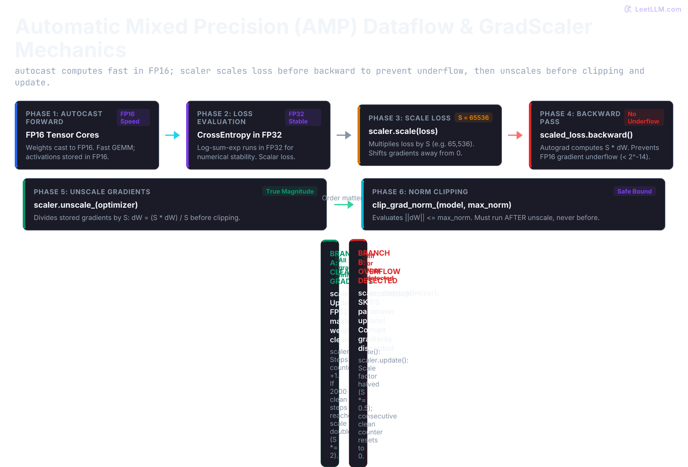
autocast executes forward passes in FP16/BF16 while maintaining FP32 master weights. GradScaler shifts loss by scale factor S before backward() to prevent underflow. Gradients must be unscaled before clipping. Clean steps update weights, while overflow events skip updates and halve the scale factor.When training with bfloat16 on compatible hardware, the format's 8-bit exponent matches float32's dynamic range (), which eliminates gradient underflow. Consequently, pure bfloat16 training typically omits GradScaler entirely.
1import torch
2from torch import nn
3
4torch.manual_seed(7)
5device = torch.device("cuda" if torch.cuda.is_available() else "cpu")
6use_amp = device.type == "cuda"
7model = nn.Linear(2, 2).to(device)
8optimizer = torch.optim.SGD(model.parameters(), lr=0.1)
9loss_fn = nn.CrossEntropyLoss()
10xb = torch.tensor([[1.2, 0.8], [-1.0, -0.7]], device=device)
11yb = torch.tensor([1, 0], dtype=torch.long, device=device)
12scaler = torch.amp.GradScaler("cuda", enabled=use_amp)
13before = [parameter.detach().clone() for parameter in model.parameters()]
14
15optimizer.zero_grad(set_to_none=True)
16with torch.amp.autocast("cuda", dtype=torch.float16, enabled=use_amp):
17    logits = model(xb)
18    loss = loss_fn(logits, yb)
19
20scaler.scale(loss).backward()
21scaler.unscale_(optimizer)
22grad_norm = torch.nn.utils.clip_grad_norm_(model.parameters(), max_norm=1.0)
23scaler.step(optimizer)
24scaler.update()
25
26changed = any(not torch.equal(old, new) for old, new in zip(before, model.parameters()))
27print("AMP enabled:", use_amp)
28print("finite loss:", bool(torch.isfinite(loss)))
29print("finite unscaled gradient norm:", bool(torch.isfinite(grad_norm)))
30print("parameters changed:", changed)1AMP enabled: False
2finite loss: True
3finite unscaled gradient norm: True
4parameters changed: TrueOn CPU, enabled=False acts as a transparent pass-through: autocast is a no-op, scaler.scale(loss) returns the raw loss, unscale_ does nothing, and scaler.step(optimizer) executes optimizer.step() directly.
Graph compilation after eager verification
torch.compile optimizes PyTorch execution by capturing Python operations into a computational graph via TorchDynamo and compiling them into fused kernels via TorchInductor.[15][16]
Compilation accelerates execution, but it doesn't fix logic errors. If your eager loop has misordered optimizer steps, unhandled NaN gradients, or leaky validation splits, torch.compile will simply compile those bugs. Always verify your loop's eager execution and numerical correctness before applying compilation.
We test graph capture below using backend="eager", which runs the captured graph through standard PyTorch operations to verify graph validity without requiring a GPU compiler.
1import torch
2from torch import nn
3
4torch.manual_seed(0)
5eager = nn.Linear(2, 2)
6compiled = torch.compile(eager, backend="eager")
7ticket = torch.tensor([[1.2, 0.8]])
8
9eager_logits = eager(ticket)
10compiled_logits = compiled(ticket)
11print("compiled module:", type(compiled).__name__)
12print("logits match eager:", torch.allclose(eager_logits, compiled_logits))1compiled module: OptimizedModule
2logits match eager: TrueIf compiled outputs diverge from eager outputs, look for unsupported Python control flow or in-place tensor mutations. Graph breaks hurt runtime performance rather than producing numerical errors. Profile steady-state loop iterations separately to exclude one-time compilation warm-up overhead.[17]
Artifacts and audit receipts for the training run
Before deploying a model to production, assemble an audit trail verifying training integrity:
| Artifact component | Operational importance |
|---|---|
| Model architecture and optimizer config | Documents exact model hyperparameters and optimizer settings. |
| Epoch loss trajectories (train vs validation) | Distinguishes steady optimization from overfitting or divergence. |
| Selected checkpoint and metric criteria | Identifies the exact epoch weights promoted to serving. |
| Feature schema and label mappings | Ensures production feature pipelines match training tensor contracts. |
| Dataset split identifier and git commit | Guarantees auditability and prevents data leakage across splits. |
Practice: break and repair the loop
Solidify your understanding of loop mechanics by intentionally breaking individual steps in our runnable examples. Predict the failure symptom before running each test:
- In
03-one-update.py, comment outoptimizer.step(). Predict whetherchanged by stepremainsTrue. - In
04-zero-grad.py, invokebackward()three times before clearing gradients. Predict the resulting gradient magnitude. - In
07b-checkpoint-snapshot.py, replacecopy.deepcopy(...)withmodel.state_dict(). Predict which assertion fails when live weights change. - In
08-train-eval-modes.py, leave the model in training mode during the second pair of predictions. Predict whether repeated forward passes match. - In
12-amp-ordering-pattern.py, explain why callingscaler.unscale_(optimizer)beforeclip_grad_norm_is mandatory. - In
13-compile-after-eager.py, modify an eager weight after callingtorch.compileand predict whether compiled output changes.
Expected observations
- Without
optimizer.step(), autograd populates.grad, but parameter values remain unchanged (changed by step: False). - The gradient accumulates to
6.0: each backward pass adds another derivative of2.0into.grad. copied state stayed at zeroevaluates toFalse. Both dictionaries reference live parameter storage, so both follow the weight update.- Dropout zeroes random neurons on each pass in training mode, causing repeated forward passes on identical inputs to disagree.
GradScalermultiplies loss by before backpropagation. Clipping beforeunscale_compares againstmax_norm, effectively clipping true gradients at and eliminating updates.torch.compilewraps the original module rather than copying weights, so in-place edits to eager parameters reflect immediately in compiled outputs.