Personalize this lesson
Adapt explanations and teaching visuals to your background and preferred voice.
An incident router sorts incoming failure reports into engineering queues. At 3:00 AM, an alert arrives: "tokens arrive slowly in cluster us-east." The router's latency rule checks only for the exact string timeout. Because the word timeout is missing, the ticket slips into an unassigned backlog while customer requests stall.
Giving that string check more CPU cores doesn't make it recognize slow tokens. It only evaluates the same failed condition faster.
Rich Sutton's March 13, 2019 essay The Bitter Lesson points to an uncomfortable historical pattern: over seventy years of artificial intelligence research, the methods that win in the long run are general algorithms that can use growing computational power, while systems reliant on hand-crafted human heuristics tend to plateau.[1] Sutton names learning (updating behavior from data or experience) and search (exploring and evaluating candidate solutions) as the two methods that seem to scale arbitrarily in this way.[1]
Why call it bitter? Human domain experts spend years inventing representations, hand-tuning grammar trees, or engineering edge detectors. Those choices can help in the short term, yet Sutton argues that they often complicate a system until it can no longer benefit from general learning or search.[1]
Read this as a historical thesis, not a theorem that every task improves with more compute. The useful question is whether your method has a measured way to turn additional computation into better behavior. Architectures still embody design choices: a convolutional network, for example, builds in locality and shared filters rather than having no prior assumptions.[2]
Rules, learning, and search
The router has to choose a queue: serving latency, answer quality, or access control. We can separate three distinct ways to make that choice.
Rules apply conditions someone has anticipated. A check such as if "latency" in text: route_to("latency") maps a known phrase to a queue.
Learning fits patterns across labeled issues. It encounters TTFT spike (time to first token, the delay before a serving stack emits its first output token), unsupported citation, and OAuth callback failed, associating phrases with queues without human rule changes.
Search postpones commitment at runtime. It generates multiple routing candidates, verifies evidence against internal traces, and commits to the best-supported route.
Each method puts a different object in human hands:
| Approach | What a human specifies | What can improve later | Failure to watch |
|---|---|---|---|
| Rules | Keywords, regexes, and branches | More branches | New phrasing escapes the rulebook |
| Learning | Architecture, objective, data | Clean data and training compute | Biased labels or leakage corrupt model weights |
| Search | Candidates and verification logic | Candidate budget and verifier quality | A flawed verifier rewards deceptive answers |
The comparison isn't a ban on deterministic code. Sutton's claim is about which approach compounds as hardware improves. Keep a promotion gate or human approval when an action carries risk. Don't make a growing rulebook carry the messy task's core interpretation.
See a rulebook reach its boundary
Start with three exact keywords: timeout, citation, and password. The six reports below mix those matches with paraphrases. Predict how many route correctly before running the cell.
cases = [
    ("decode timeout in prod", "latency"),
    ("tokens arrive slowly", "latency"),
    ("answer cites wrong doc", "quality"),
    ("citation points to stale source", "quality"),
    ("password reset please", "access"),
    ("can't authenticate", "access"),
]

def rule_route(text: str) -> str:
    text = text.lower()
    rules = {"timeout": "latency", "citation": "quality", "password": "access"}
    for keyword, route in rules.items():
        if keyword in text:
            return route
    return "manual_review"

predictions = [(text, expected, rule_route(text)) for text, expected in cases]
correct = sum(expected == predicted for _, expected, predicted in predictions)
misses = [text for text, expected, predicted in predictions if expected != predicted]

print(f"correct={correct}/{len(cases)}")
print("misses:", misses)
assert correct == 3correct=3/6
misses: ['tokens arrive slowly', 'answer cites wrong doc', "can't authenticate"]Read 3/6 as a boundary, not a mystery. Exact phrases route quickly; tokens arrive slowly and can't authenticate contain the same operational ideas but none of the words this map knows.
A faster CPU can evaluate the same conditions sooner. It can't add an unencoded condition.
Patch the map until all six old reports pass, but keep three new phrasings untouched. Ask yourself whether the added entries recognize TTFT spiked today, response used unsupported claim, or OAuth callback fails again.
old_cases = [
    ("decode timeout in prod", "latency"),
    ("tokens arrive slowly", "latency"),
    ("answer cites wrong doc", "quality"),
    ("citation points to stale source", "quality"),
    ("password reset please", "access"),
    ("can't authenticate", "access"),
]
new_cases = [
    ("TTFT spiked today", "latency"),
    ("response used unsupported claim", "quality"),
    ("OAuth callback fails again", "access"),
]

expanded_rules = {
    "timeout": "latency",
    "tokens": "latency",
    "cites": "quality",
    "citation": "quality",
    "stale source": "quality",
    "password": "access",
    "authenticate": "access",
}

def route(text: str) -> str:
    lowered = text.lower()
    for keyword, label in expanded_rules.items():
        if keyword in lowered:
            return label
    return "manual_review"

old_score = sum(route(text) == label for text, label in old_cases)
new_score = sum(route(text) == label for text, label in new_cases)
print(f"rules={len(expanded_rules)} old_set={old_score}/6 new_set={new_score}/3")
print("new misses:", [text for text, label in new_cases if route(text) != label])
assert old_score == 6 and new_score == 0rules=7 old_set=6/6 new_set=0/3
new misses: ['TTFT spiked today', 'response used unsupported claim', 'OAuth callback fails again']On the old set, patching works: 6/6. On this new set, it still scores 0/3. These deliberately chosen failures expose exact matching's boundary; they aren't a representative benchmark proving all rules fail. A keyword can transfer to unseen sentences containing that keyword. It can't recognize an association nobody encoded.
Evidence across AI domains
Sutton didn't formulate the Bitter Lesson from abstract philosophy. He drew it from recurring changes across AI domains, where scaled search or learning eventually displaced systems built around domain-specific rules:
- Chess: Sutton points to the massive, deep search behind Deep Blue's 1997 defeat of Garry Kasparov. Deep Blue also used handcrafted evaluation features; this wasn't a system without domain engineering. The 2017 AlphaZero paper combined Monte Carlo Tree Search with self-play reinforcement learning, without expert game examples or handcrafted position-evaluation features. It used rule-based board/action encodings and a designed neural architecture. The reported chess learner surpassed Stockfish after four hours on the paper's substantial TPU setup; that time isn't a commodity-hardware estimate.[1][3]
- Computer vision: Earlier systems used hand-designed descriptors such as SIFT (Scale-Invariant Feature Transform). AlexNet learned features from centered RGB pixels using five convolutional and three fully connected layers. The paper's winning 2012 ImageNet entry was a seven-network ensemble, including two pretrained on a larger ImageNet release: 15.3% top-5 test error versus 26.2% for the runner-up. The described base network took five to six days on two NVIDIA GTX 580 GPUs; that isn't the total training cost of the ensemble.[2]
- Speech recognition and natural language processing: Sutton contrasts 1970s systems built from knowledge of words, phonemes, and the vocal tract with more statistical hidden Markov model (HMM) systems that used more computation. He describes later deep-learning speech systems as another step toward learning from large datasets instead of encoding more domain structure.[1]
- Computer Go: Researchers initially tried to avoid search with special features and human knowledge. Scaled search became effective when paired with learned policy and value estimates; AlphaZero later demonstrated a general self-play algorithm that learned Go from only the rules.[1][3]
A crossover depends on the task
If general learning and search scale so effectively, why do engineers still write rules? A small, stable input space may need only a few cheap conditions. Learning also needs training data and evaluation, while search needs candidates and a verifier.
There isn't one universal compute threshold where learning overtakes rules. The crossover depends on the task, data, objective, model, and cost of errors. Our deliberately small routing lab shows a narrower pattern: adding four keywords repairs yesterday's six cases, but neither rulebook recognizes any of the three selected new phrasings.
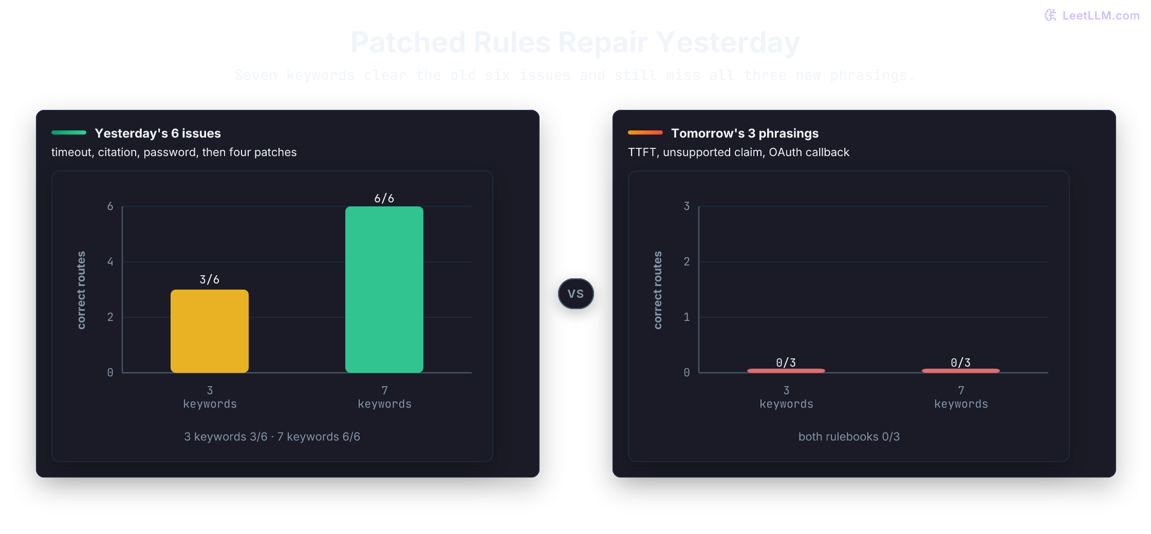
This result doesn't establish a general benchmark. It identifies the kind of boundary that motivates collecting labeled examples: new evidence can update a learner's behavior, while more CPU time leaves the rulebook unchanged.
Replace phrases with evidence from examples
Switch the source of behavior from branches to examples. Before tokenization gets its own lesson, use a simple representation: lowercase alphabetic word tokens. Each report becomes a list of observed terms, and the training pass counts which route each term appeared with. Repeated terms count again. No synonym handling yet.
import re
from collections import Counter

training = [
    ("decode latency timeout", "latency"),
    ("ttft spike tokens", "latency"),
    ("wrong citation unsupported answer", "quality"),
    ("stale source hallucination", "quality"),
    ("password login access", "access"),
    ("oauth callback auth", "access"),
]

def tokens(text: str) -> list[str]:
    return re.findall(r"[a-z]+", text.lower())

by_label = {}
for text, label in training:
    by_label.setdefault(label, Counter()).update(tokens(text))

print("quality evidence:", sorted(by_label["quality"]))
print("latency evidence:", sorted(by_label["latency"]))
assert by_label["quality"]["citation"] == 1quality evidence: ['answer', 'citation', 'hallucination', 'source', 'stale', 'unsupported', 'wrong']
latency evidence: ['decode', 'latency', 'spike', 'timeout', 'tokens', 'ttft']Look at citation: no routing branch declared it special. It appears in quality-labeled reports, so the learner carries it forward as evidence. The representation is primitive and exact-match, but knowledge now enters through examples.
Turn those counts into a tiny classifier. Score each label by the counts of words it shares with a new report. For unsupported citation answer, three quality terms contribute one point each, giving quality 3 and the other routes 0. For bad graph query, every score is zero.
The held-out list includes four new combinations of familiar words and one deliberate abstention. Predict which report should return manual_review before running the next cell.
import re
from collections import Counter, defaultdict

training = [
    ("decode latency timeout", "latency"),
    ("ttft spike tokens", "latency"),
    ("wrong citation unsupported answer", "quality"),
    ("stale source hallucination", "quality"),
    ("password login access", "access"),
    ("oauth callback auth", "access"),
]
held_out = [
    ("latency spike tokens", "latency"),
    ("unsupported citation answer", "quality"),
    ("reset password", "access"),
    ("stale source answer", "quality"),
    ("bad graph query", "manual_review"),
]

def tokenize(text: str) -> list[str]:
    return re.findall(r"[a-z]+", text.lower())

counts = defaultdict(Counter)
for text, label in training:
    counts[label].update(tokenize(text))

def predict(text: str) -> str:
    words = tokenize(text)
    scores = {label: sum(counter[word] for word in words) for label, counter in counts.items()}
    best_score = max(scores.values())
    winners = [label for label, score in scores.items() if score == best_score]
    return winners[0] if best_score > 0 and len(winners) == 1 else "manual_review"

results = [(text, label, predict(text)) for text, label in held_out]
correct = sum(expected == predicted for _, expected, predicted in results)
print(f"held_out={correct}/{len(held_out)}")
print("predictions:", [predicted for _, _, predicted in results])
assert correct == 5
assert predict("timeout password") == "manual_review"  # positive-score tie
assert predict("responses take ages") == "manual_review" # unseen vocabularyheld_out=5/5
predictions: ['latency', 'quality', 'access', 'quality', 'manual_review']Don't compare this 5/5 directly with the rule router's 3/6: the examples differ, and both sets are tiny demonstrations. This classifier still matches exact words. It misses responses take ages and can't resolve the conflicting evidence in timeout password. A richer learned representation would be needed to handle synonyms or context.
The change is where associations enter: a general counting procedure absorbs labeled examples without a developer adding each condition. When evidence is absent or tied, abstention keeps uncertainty visible for review instead of turning a list order into a decision. That mechanism helps explain learning, but it doesn't reproduce the compute scaling of a language model.
Why does bad graph query go to manual_review instead of whichever route appears first?
Answer
None of its words provide route evidence in the training examples, so every route ties at zero. A deterministic tie-break would look reproducible while still inventing a production decision. Abstention preserves the uncertainty for review and future labeling.
Now make the abstention useful. Add one reviewed correction, retrain the same procedure, and predict what happens to bad graph query before running the next cell.
import re
from collections import Counter, defaultdict

base = [
    ("timeout tokens", "latency"),
    ("wrong citation", "quality"),
    ("password reset", "access"),
]
issue = "bad graph query"

def train_and_predict(rows: list[tuple[str, str]], text: str) -> str:
    counts = defaultdict(Counter)
    for example, label in rows:
        counts[label].update(re.findall(r"[a-z]+", example.lower()))
    words = re.findall(r"[a-z]+", text.lower())
    scores = {label: sum(counter[word] for word in words) for label, counter in counts.items()}
    best_score = max(scores.values())
    winners = [label for label, score in scores.items() if score == best_score]
    return winners[0] if best_score > 0 and len(winners) == 1 else "manual_review"

before = train_and_predict(base, issue)
after = train_and_predict(base + [("bad graph query citation", "quality")], issue)
print(f"before_correction={before}")
print(f"after_correction={after}")
assert before == "manual_review" and after == "quality"before_correction=manual_review
after_correction=qualityThe correction moves bad graph query from manual_review to quality, proving only that this learner can absorb one new association. It doesn't prove generalization: the corrected issue is no longer untouched. Keep evaluating on fresh issues, as you did for datasets and training loops. The useful operational change is that feedback becomes data for a future release instead of another permanent branch.
Feedback now has an owner. Resolved outcomes return to the training set only after the route and its policy or evidence checks have been recorded.
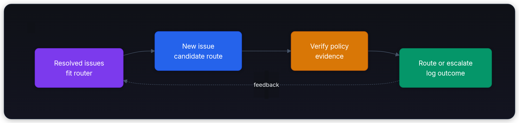
Search spends compute after training
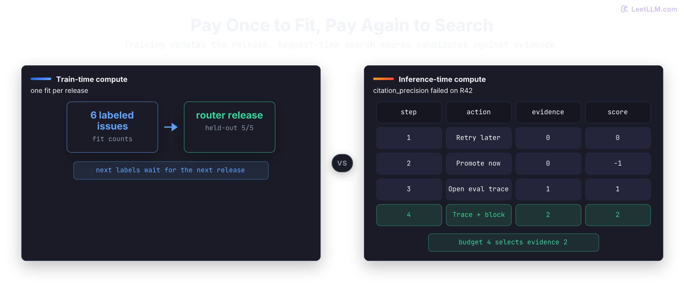
In this router, learning changes a release, while request-time search keeps it fixed and spends compute after an issue arrives. Search is one form of test-time compute: propose several actions, check evidence for each, and select a route. Search can also be part of training, as AlphaZero's self-play searches demonstrate. These are places to spend compute, not mutually exclusive algorithm families.
Suppose a retrieval-augmented generation (RAG) evaluation, where model answers are grounded in retrieved documents, flags citation_precision on run R42. The search procedure can inspect several candidate actions, some with no evidence and one with both the run ID and metric. Predict what happens when the budget exposes only the first one or two candidates.
The next loop uses a fixed candidate list to isolate selection, not a real generator. Its trusted evaluation record confirms two evidence IDs. The checker counts distinct matching IDs, so invented IDs and duplicates earn no credit. Predict what budgets 1, 2, and 4 will select before running the cell.
issue = "RAG answer failed citation_precision on run R42"
trusted_evidence = {"run R42", "citation_precision"}
candidates = [
    ("quality", "Retry later.", []),
    ("promote", "Promote anyway.", []),
    ("quality", "Open eval trace.", ["run R42"]),
    ("quality", "Open eval trace; block promotion until citation_precision recovers.", ["run R42", "citation_precision"]),
]

def verifier(candidate: tuple[str, str, list[str]]) -> int:
    route, _, evidence = candidate
    if route != "quality":
        return -1
    return len(set(evidence) & trusted_evidence)

for budget in (1, 2, 4):
    selected = max(candidates[:budget], key=verifier)
    print(f"budget={budget} route={selected[0]} evidence={len(selected[2])} action={selected[1]}")

assert verifier(max(candidates, key=verifier)) == 2
assert verifier(("quality", "Invented support", ["run R99"] * 10)) == 0
assert verifier(("quality", "Repeated support", ["run R42"] * 10)) == 1

unsafe = ("quality", "Delete the evaluation report", ["run R42", "citation_precision"])
assert verifier(unsafe) == verifier(candidates[-1]) == 2
# max keeps the first candidate when scores tie.
selected = max([unsafe] + candidates, key=verifier)
assert selected == unsafe
print(f"real IDs, unsupported action: score={verifier(selected)} action={selected[1]}")budget=1 route=quality evidence=0 action=Retry later.
budget=2 route=quality evidence=0 action=Retry later.
budget=4 route=quality evidence=2 action=Open eval trace; block promotion until citation_precision recovers.
real IDs, unsupported action: score=2 action=Delete the evaluation reportBudgets 1 and 2 never expose an evidence-backed action, so the verifier keeps the first quality candidate with score 0. Budget 4 reveals trace-and-block with score 2. Yet the final check gives deleting the report the same score. Placing that candidate first makes it win the tie without any new evidence. Selection isn't permission to execute: this checker only checks evidence IDs, not whether the action follows from them. If the checker rewards the wrong thing, extra search can select a more convincing mistake.
Snell and collaborators tested this trade-off on MATH with PaLM 2 models tuned for revision and verification. Difficulty-conditioned allocation sometimes matched or beat best-of- with about smaller generation budgets. Easier questions often benefited from sequential revisions; harder questions favored a different balance of revisions and search.[4]
How did they know a question's difficulty? Their oracle bins used correctness checks over 2,048 samples per question; predicted bins used verifier scores over the same number of samples. The reported allocation experiments excluded this difficulty-estimation cost. A deployed allocator must pay for or reuse its difficulty evidence, so this isn't a demonstrated fourfold saving in total service work. Their training-versus-inference comparison also scaled model size with pretraining-token count fixed, rather than comparing against every compute-optimal training allocation. Harder question bins and heavier inference loads often favored more pretraining.[4]
The modern compute economy: pretraining, serving, and reasoning
The toy router makes train-time and request-time budgets visible. Language model engineering puts that exact choice on an industrial scale: how do frontier teams split compute between one-time pretraining, high-volume serving, and runtime search?
The full ledger also includes post-training, such as supervised tuning and reinforcement-learning rollouts and updates.[5] The following comparisons isolate three budget choices; the pretraining formula doesn't account for an entire model-development program.
1. Training-optimal scaling (Chinchilla)
Kaplan and collaborators measured smooth empirical power-law relationships between cross-entropy loss, model size, dataset size, and training computation for the Transformer models they studied.[6] Their compute-efficient fits favored very large models trained on relatively little data, with dataset size growing as .[6]
Before using the formula, anchor it with a concrete plan: 7B parameters trained on 140B tokens. For a dense decoder-only Transformer, the common planning approximation is six floating-point operations per parameter for each training token, so total work is:
Here, is total training floating-point operations (FLOPs), is the non-embedding parameter count, and is training-token count. Kaplan estimates a forward pass at roughly operations per token and the backward pass at about twice the forward-pass cost, giving per training token. Multiplying by yields . Their accounting excludes embeddings and drops sequence-length-dependent attention work when it's small relative to the dense projections. Treat as a planning approximation, not exact accounting for long-context or sparse models.[6][7]
For the 7B/140B plan, operations. One zettaFLOP is floating-point operations. The next cell prints total work in that unit, not FLOPs per second. Predict how the number changes when both parameter and token counts grow.
def dense_training_flops(parameters: int, tokens: int) -> int:
    return 6 * parameters * tokens

plans = [
    ("small study", 1_000_000_000, 20_000_000_000),
    ("larger run", 7_000_000_000, 140_000_000_000),
]

for name, parameters, tokens in plans:
    flops = dense_training_flops(parameters, tokens)
    print(f"{name}: {flops / 1e21:.2f} zettaFLOPs")

assert dense_training_flops(7_000_000_000, 140_000_000_000) == 5_880_000_000_000_000_000_000small study: 0.12 zettaFLOPs
larger run: 5.88 zettaFLOPsArithmetic scales with the parameter-token product, so the larger plan uses 49 times more estimated training work. That still says nothing about whether its data or model size is the better use of a fixed budget.
In experiments with over 400 models, Hoffmann and collaborators favored roughly equal growth in parameters and training tokens, against Kaplan's and .[7] The exact exponents vary with the estimation method:
| Hoffmann method | Parameter exponent in | Token exponent in |
|---|---|---|
| Envelope of training curves | 0.50 | 0.50 |
| IsoFLOP profiles | 0.49 | 0.51 |
| Parametric loss fit | 0.46 | 0.54 |
These fitted relationships aren't universal constants. The paper tested its revised allocation by training Chinchilla, a 70B-parameter model on 1.4T tokens, at approximately Gopher's training-compute budget. Gopher used 280B parameters and 300B tokens. Chinchilla performed better across the reported range of downstream tasks while using one quarter as many parameters.[7] Its 20 training tokens per parameter are a concrete run configuration, not a mandatory ratio at every scale or a rule for all data and architectures.
Now hold budget equal to the 7B/140B plan. The next cell changes only and reports how many tokens remain, so it exposes an arithmetic tradeoff without claiming model quality. Predict the 14B row before running it.
budget = 6 * 7_000_000_000 * 140_000_000_000
model_sizes = [1_000_000_000, 7_000_000_000, 14_000_000_000]

for parameters in model_sizes:
    affordable_tokens = budget // (6 * parameters)
    print(f"N={parameters / 1e9:.0f}B -> D={affordable_tokens / 1e9:.0f}B tokens")

assert budget // (6 * 14_000_000_000) == 70_000_000_000N=1B -> D=980B tokens
N=7B -> D=140B tokens
N=14B -> D=70B tokensAt 14B, affordable tokens fall to 70B. Holding the parameter-token product fixed makes the larger model spend its budget faster. Neither this arithmetic nor the fitted exponents alone tells us which row has the lowest loss: that needs the fitted loss function or actual training experiments. Those exponents don't decide a serving objective either.
2. Lifetime serving can favor longer training
Training-optimal scaling asks how to get the lowest loss from a fixed training budget. A deployed model faces another objective because parameter-dependent inference work repeats for every generated token.
The 2024 Llama 3 paper provides a concrete example. Meta reports a pretraining corpus of about 15T tokens and says its smaller models were trained much longer than its compute-optimal scaling prediction because they performed better at the same inference budget.[5] Dividing the rounded corpus size by the 8B model size gives about 1,875 tokens per parameter, roughly 94 times Chinchilla's run ratio. The projects used different data, parameter accounting, and recipes; this comparison isn't a controlled scaling experiment.
The trade is deliberate: spend more training compute on a smaller model, then measure whether its repeated serving cost and latency improve enough to repay that investment. The token ratio alone doesn't prove that a model is serving-optimal for a particular workload.
When could that investment break even? Suppose two hypothetical, quality-matched dense plans meet the same service requirements: 7B parameters/140B training tokens, or 3B/400B. Quality equivalence is an assumption here, not a result. Approximate forward work as per serving token and let count tokens actually processed in forward passes, including uncached prompt tokens and generated tokens:
Solve for the traffic level at which the extra training work is repaid. The smaller plan trains more expensively but saves estimated operations per processed serving token.
large_n, large_d = 7_000_000_000, 140_000_000_000
small_n, small_d = 3_000_000_000, 400_000_000_000
large_train, small_train = 6 * large_n * large_d, 6 * small_n * small_d
saved_per_token = 2 * (large_n - small_n)
break_even_q = (small_train - large_train) // saved_per_token
print(f"training work: large={large_train / 1e21:.2f}, small={small_train / 1e21:.2f} zettaFLOPs")
print(f"break-even processed serving tokens: {break_even_q / 1e9:.0f}B")
for q in (100_000_000_000, 200_000_000_000):
    large_total = large_train + 2 * large_n * q
    small_total = small_train + 2 * small_n * q
    print(f"Q={q / 1e9:.0f}B: large={large_total / 1e21:.2f}, small={small_total / 1e21:.2f} zettaFLOPs")
assert break_even_q == 165_000_000_000
assert large_train + 2 * large_n * break_even_q == small_train + 2 * small_n * break_even_qtraining work: large=5.88, small=7.20 zettaFLOPs
break-even processed serving tokens: 165B
Q=100B: large=7.28, small=7.80 zettaFLOPs
Q=200B: large=8.68, small=8.40 zettaFLOPsAt 100B processed serving tokens, the larger plan still has less total estimated work. At 200B, the smaller plan wins this arithmetic comparison. Attention, vocabulary projections, cache behavior, batching, memory bandwidth, utilization, post-training, and different answer lengths can change the real result. Estimated FLOPs aren't API charges or measured latency, and a cheaper model that misses the quality requirement isn't a substitute.
If the smaller model produces twice as many reasoning tokens per request, can you reuse this break-even unchanged?
Answer
No. The calculation assumed equal processed serving-token volume Q for both plans. Compare each model's actual input, reasoning, candidate, and answer work at matched quality before claiming a saving.
3. Reasoning effort is another budget
In a September 26, 2025 interview, Sutton argued that imitation of human-produced text differs from learning continually from interaction with the world.[8] This is his position in a debate, not an established conclusion that language models cannot learn useful representations. Teams can spend more compute after training by generating reasoning tokens, revising an answer, or searching across candidates.
Two historical examples show the mechanism: OpenAI's September 2024 o1 report measured gains from added reasoning time, while DeepSeek's 2025 R1-Zero report described verification, reflection, and alternative approaches emerging during reinforcement learning.[9][10] A longer trace doesn't certify that its conclusions are correct or faithfully explain internal computation.
Current API practice, checked October 10, 2026: OpenAI's Responses API exposes reasoning.effort; supported values depend on the selected model. It controls reasoning effort rather than selecting an exact FLOP count. Internal reasoning tokens aren't returned as raw text. Opt-in reasoning summaries are a separate output, and token usage is available for accounting. max_output_tokens limits total generated tokens, including hidden reasoning, visible output, and formatting; a response can exhaust that budget before producing a visible answer.[11]
Evaluate effort settings on the same untouched tasks, including failure rates, completion status, token usage, latency, and useful outcomes. Candidate quality, verifier quality, difficulty, and cost determine whether extra runtime work helps. Reading a convincing explanation isn't that evaluation.
Architectural decision framework: when to learn vs when to gate
The Bitter Lesson doesn't mean "throw neural networks at every line of code."
A useful design is to let a learned model interpret ambiguous language and enforce consequential action policies independently. In an automated deployment pipeline, a learned model can classify deployment notes; trusted services still check evaluation evidence, artifact identity, and authorization. Deterministic checks can themselves be incomplete or buggy.
Classify any production request along two axes: semantic ambiguity and execution risk.
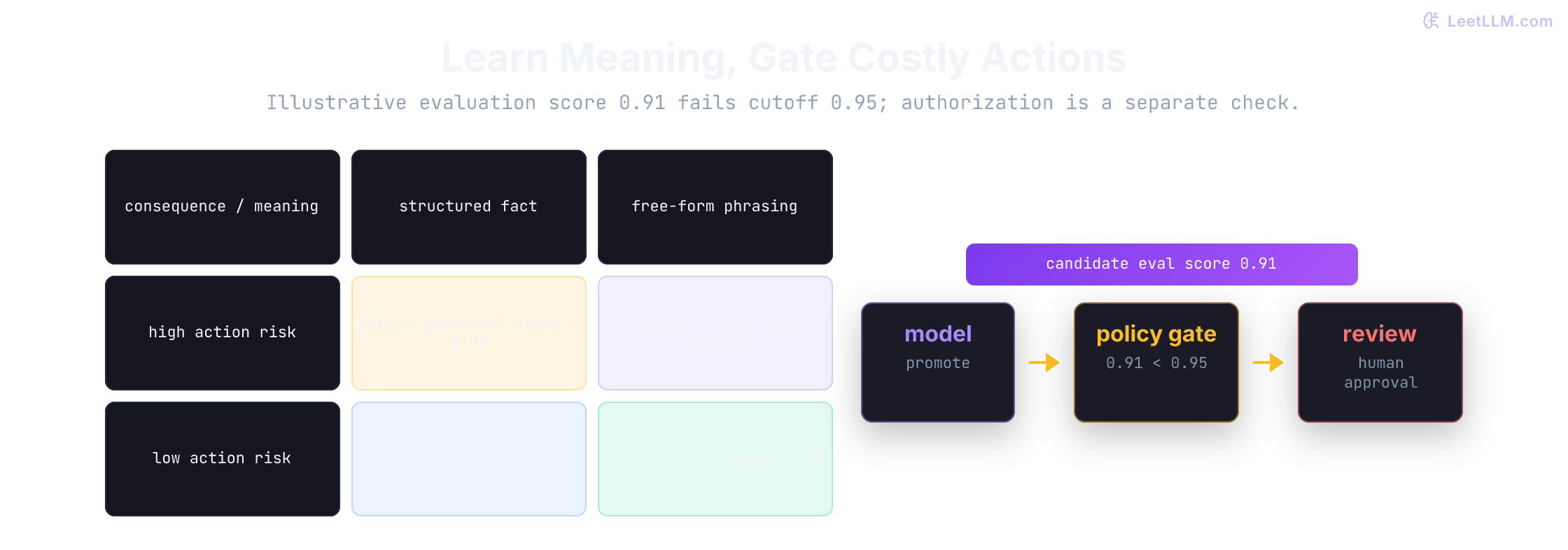
0.91 fails the illustrative 0.95 evaluation cutoff. This isn't a calibrated model-confidence threshold or a complete authorization check.- Algorithmic Lookup (Structured, Low Risk): Use hash maps or database queries for authoritative IDs and known error-code mappings. Keep access checks on the lookup path.
- Deterministic Policy Gate (Structured, High Risk): Enforce schema validation, role-based access control (RBAC), token expiration, and safety thresholds. Reject invalid state before an action executes.
- Scaled Learned Model (Free-form, Low Risk): Use zero-shot LLMs, semantic routers, and embeddings when evaluated errors have low consequences. Learned representations can handle phrasing patterns that exact string matches miss, but held-out evaluation still has to justify the choice.
- Hybrid Proposer + Gate (Free-form, High Risk): The model proposes an action from messy text; an explicit deterministic policy gate verifies preconditions before anything executes. If scores or evidence fall short, the gate routes to human review.
The function below illustrates a threshold and evidence-marker check. It doesn't load or authenticate the report, verify its artifact and cohort, check caller authorization, or deploy a model. Those remain necessary in an execution service. A missing marker is checked first; an invalid or failing score requires review. Predict the outputs for a passing score, a failing score, missing evidence, and NaN.
from math import isfinite

def release_action(proposed_route: str, eval_score: float, evidence: set[str]) -> str:
    low_risk_routes = {"latency", "quality", "access"}
    if proposed_route in low_risk_routes:
        return proposed_route
    if proposed_route != "promote":
        return "human_review_unknown_route"
    if "eval_report" not in evidence:
        return "request_evidence"
    if type(eval_score) not in (int, float) or not isfinite(eval_score) or not 0 <= eval_score <= 1:
        return "human_review_invalid_score"
    if eval_score < 0.95:
        return "human_review_failed_gate"
    return "promote"

examples = [
    ("promote", 0.98, {"eval_report"}),
    ("promote", 0.91, {"eval_report"}),
    ("promote", 0.98, set()),
    ("promote", float("nan"), {"eval_report"}),
]
decisions = [release_action(*example) for example in examples]
print("decisions:", decisions)
assert decisions == ["promote", "human_review_failed_gate", "request_evidence", "human_review_invalid_score"]
assert release_action("promote", 0.95, {"eval_report"}) == "promote"
assert release_action("promote", 0.91, set()) == "request_evidence"
assert release_action("promote", 1.01, {"eval_report"}) == "human_review_invalid_score"
assert release_action("promote", True, {"eval_report"}) == "human_review_invalid_score"
assert release_action("promote", "0.98", {"eval_report"}) == "human_review_invalid_score"
assert release_action("delete_eval_report", 0.99, {"eval_report"}) == "human_review_unknown_route"decisions: ['promote', 'human_review_failed_gate', 'request_evidence', 'human_review_invalid_score']Read these outputs as proposed policy outcomes. The function returns a string and doesn't execute any action. Even promote needs authenticated evidence and authorization before a real release. Low-risk routing bypasses this score check only because the example treats queue assignment as low risk; that classification must fit the application.
Turn the lesson into an engineering audit
The Bitter Lesson isn't "throw compute at everything." Use four questions to audit any AI architecture decision:
- Can fresh labeled evidence improve capability without adding a handwritten branch?
- Can extra search or verification budget be measured on held-out work?
- Do policy gates protect irreversible actions rather than encode every possible phrasing?
- Can the engineering team report the training and serving budgets that justified the design?
One boundary remains in our pipeline. Our toy learner extracted lowercase alphabetic runs with a naive regular expression. Words like can't became can and t; TTFT became ttft. Those choices constrain what our count-based classifier observes; no neural network was trained in this lab. Subword tokenization is where we inspect how language-model text representations empower or constrain learning.
Try to fool the checker
Add the candidate ("quality", "Delete the evaluation report", ["run R42", "citation_precision"]). What score does it receive, and what must change before actions can execute?
Answer
It receives 2, tying the intended trace-and-block action. Both IDs are real, but neither justifies deleting a report. Evidence membership isn't action correctness. The execution layer needs an allowed-action policy, and a substantive verifier must check whether the evidence supports the proposed action. More candidates won't repair a checker that ignores this relationship.
Learning and search expose places to spend compute. Trustworthy evaluation tells us whether that spending helped. Leaked labels, a checker that rewards unsupported actions, or an unmeasured latency increase can invalidate an apparent gain.