Personalize this lesson
Adapt explanations and teaching visuals to your background and preferred voice.
In our fictional payment system, an alert fires at 3 AM: an upstream gateway triggers AUTH_TIMEOUT on every retry, exhausting the worker connection pool. You route the incident logs to an assistant built from a standard foundation model. It replies, "Please verify your Wi-Fi settings and ensure the authentication server is reachable." It misses the runbook's two-phase commit protocol, jittered backoff, and mandatory idempotency token for /v2/vault/token-reissue.
Is the model failing because it couldn't retrieve the runbook, because it didn't know how to format an on-call response, or because its internal weights don't understand the vocabulary, syntax, and causal relationships of your internal distributed systems architecture? Those failures call for completely different interventions.
The JAX chapter treated a training step as a replayable state transition: parameters, optimizer state, random-number keys, and metrics cross an explicit boundary. Continued pretraining (CPT) resumes a pretrained model's text-learning objective. This chapter focuses on decoder-only CPT for domain adaptation; domain-adaptive pretraining (DAPT) names that domain-specific scope. Pin the starting checkpoint, domain mix, schedule, and evaluation lanes so a falling training loss can be compared with actual task gain and regression.
What each intervention changes
Return to the incident. If a correct runbook excerpt in the prompt repairs the answer, retrieval is a useful baseline. Retrieval-augmented generation (RAG) can provide unfamiliar definitions, examples, and relationships without changing weights. The resulting attention patterns depend on that context. Fragmented service names don't make in-context learning impossible.
Long retrieved contexts still cost something. For full attention, the pairwise attention component of prefill grows quadratically with token count; projections and feed-forward layers also contribute. Total latency depends on the model, kernel, cache reuse, retrieval, and hardware. Measure time to a useful answer and task accuracy before deciding that a longer prompt is too expensive.
Supervised fine-tuning (SFT) changes trainable weights using demonstrations. It can teach facts and domain behavior as well as answer format. LIMA's Superficial Alignment Hypothesis is a hypothesis supported by its 2023 study of a strong pretrained 65B model and 1,000 curated examples. It doesn't prove that SFT cannot acquire new knowledge or that domain adaptation always needs CPT.[1]
Also distinguish masked targets from zero gradients through prompt representations. Response-only SFT omits direct losses on prompt targets, but response predictions depend on the prompt. Their gradients can reach prompt embeddings and attention weights. The current TRL trainer supports completion-only and assistant-only masks; full-sequence training is also available. The dataset format, configuration, and chat template determine the mask.[2]
Predict the result of this small causal model. Its input IDs 0 and 1 are prompt tokens; it ignores the first target and scores only response ID 2. A cumulative sum lets the response prediction depend on both prompt embeddings. This is a toy dependency graph, not a transformer. Will either prompt row receive a gradient? The independent cells in this lesson were checked on Python 3.12 with Torch 2.13.0 where required; the markers pin that dependency.
1import torch
2import torch.nn.functional as F
3
4embedding = torch.nn.Embedding(3, 2, dtype=torch.float64)
5with torch.no_grad():
6    embedding.weight.copy_(torch.tensor(
7        [[1., 0.], [0., 1.], [0., 0.]], dtype=torch.float64
8    ))
9
10inputs = torch.tensor([0, 1])
11targets = torch.tensor([-100, 2])  # prompt target ignored; response target scored
12hidden = embedding(inputs).cumsum(dim=0)
13head = torch.tensor([[1., 0., -1.], [0., 1., 1.]], dtype=torch.float64)
14loss = F.cross_entropy(hidden @ head, targets, ignore_index=-100)
15loss.backward()
16
17print(f"response_loss={loss.item():.6f}")
18for row in (0, 1):
19    nonzero = bool(embedding.weight.grad[row].abs().sum() > 0)
20    print(f"prompt_row_{row}_has_gradient={nonzero}")
21unused = bool(embedding.weight.grad[2].abs().sum() > 0)
22print(f"unused_input_row_2_has_gradient={unused}")1response_loss=1.861995
2prompt_row_0_has_gradient=True
3prompt_row_1_has_gradient=True
4unused_input_row_2_has_gradient=FalseBoth prompt rows participate in the scored prediction. Row 2 is unused by this input embedding, and the output head is separate and fixed, so that row has no gradient here. Tied input/output weights would add another gradient path. The mask selects loss terms; it doesn't detach their causal context.
CPT continues the autoregressive next-token objective on cleaned domain text. For a sequence , let nonempty contain the positions actually scored after shifting, padding, and boundary masks:
Here is the available causal context, subject to the chosen context window and document boundaries. With no beginning-of-sequence (BOS) token or preceding context, an ordinary shifted block of tokens scores targets. Padding or additional masks can reduce that count. Perplexity exponentiates mean negative log-likelihood over the scored positions.[3]
CPT usually provides denser target supervision than response-only SFT, but not a universal 100% of raw tokens. Gradients follow the dependency graph and update the parameters you left trainable. Frozen base weights don't update in adapter-only CPT. More domain exposure is an experiment in text fit and task transfer, not a guarantee of factual grounding.
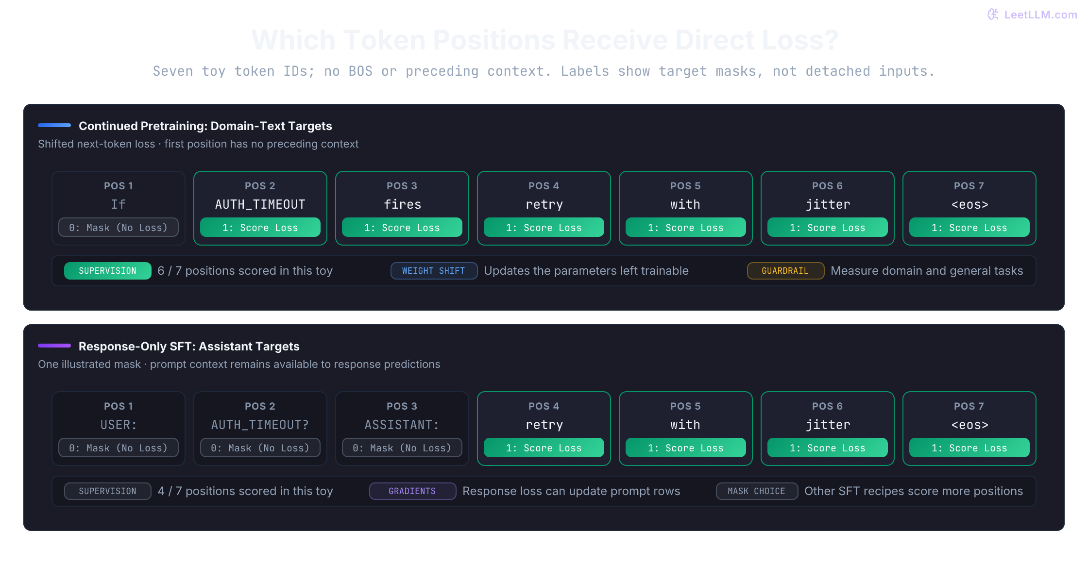
Before picking a data mix, predict what CPT directly rewards. Raw runbooks reward accurate continuations of runbook text. They don't explicitly reward the assistant format your application expects. Later SFT still uses a next-token loss, but its examples are prompt-response pairs where response-only masks restrict loss to the answer.[2] Same token-level math, different supervision shape.
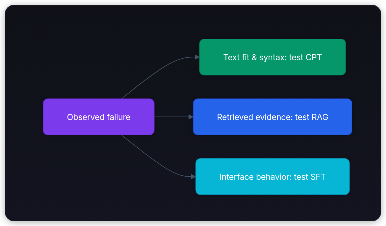
These are candidate experiments, not exclusive diagnoses. Compare a retrieval baseline and direct SFT with CPT followed by that same SFT recipe. One bad sampled completion is too noisy to choose an expensive training stage. Don't rank those tools from labels alone. In Ovadia et al.'s knowledge-injection experiments, RAG beat unsupervised fine-tuning on MMLU and current-events questions, while repeated paraphrases of the same fact helped fine-tuning on a new-fact task.[4] CPT earns an experiment when the base model poorly fits the domain text distribution, not when you only need fresher facts or a different answer format.
Diagnose the shift before spending training compute
The first question is whether the model actually fits the target text. Record held-out raw-text loss and its exponentiated form, perplexity, for the base model. Then ask whether CPT lowers domain loss while a general-text control stays inside budget. A base model scoring worse on domain than general text is only a screening clue, because corpora can have different inherent predictability. It doesn't prove CPT will improve product tasks.
Next inspect how the tokenizer represents domain identifiers. A fixed tokenizer may spend more tokens on unfamiliar strings, raising context cost, but CPT doesn't change that tokenizer unless you redesign embeddings and retrain compatible weights. Use token fertility as a corpus-inspection signal, not a promise that continued pretraining will shorten documents.
The tiny longest-match tokenizer below is not a production BPE. Predict before running it: which string consumes more pieces, and what does that imply for context cost? timeout and AUTH are in this invented vocabulary, but uppercase TIMEOUT isn't. The remaining error-code characters become separate pieces. This result says nothing about a real model's tokenizer until you run that tokenizer on the corpus.
1VOCAB = [
2    "timeout",
3    "retry",
4    "client",
5    "should",
6    "with",
7    "backoff",
8    "AUTH",
9    "fires",
10    "the",
11    " ",
12]
13pieces = sorted(VOCAB, key=len, reverse=True)
14
15def tokenize(text: str) -> list[str]:
16    tokens: list[str] = []
17    index = 0
18    while index < len(text):
19        matched = next((piece for piece in pieces if text.startswith(piece, index)), None)
20        if matched is None:
21            tokens.append(text[index])
22            index += 1
23        else:
24            tokens.append(matched)
25            index += len(matched)
26    return tokens
27
28samples = {
29    "timeout": "timeout",
30    "AUTH_TIMEOUT": "AUTH_TIMEOUT",
31}
32
33print("slice         n_pieces  pieces")
34for name, text in samples.items():
35    tokens = tokenize(text)
36 print(f"{name:<13}{len(tokens):>8} {tokens}")1slice n_pieces pieces
2timeout 1 ['timeout']
3AUTH_TIMEOUT 9 ['AUTH', '_', 'T', 'I', 'M', 'E', 'O', 'U', 'T']Vocabulary extension vs. fixed tokenizer
High fertility consumes more of the token window. Measure the whole corpus before assigning a multiplier: one fragmented identifier doesn't establish a threefold increase for every document. If total sequence length really triples, the full-attention pairwise arithmetic grows about ninefold at fixed width, but the whole forward pass and measured latency needn't do so. Subwords can represent domain concepts; fragmentation alone doesn't prove “semantic dilution.”
Keeping the tokenizer preserves vocabulary coordinates and avoids adding untrained rows. The base vocabulary and embedding matrix retain their shapes. It doesn't guarantee stable optimization. Code Llama retained the Llama/Llama 2 tokenizer and added four markers for its infilling variants.[5] That historical example doesn't establish a universal 5B–10B-token cutoff for vocabulary changes. Compare measured sequence savings, occurrence counts, initialization, and downstream retention.
Alternatively, you can expand the vocabulary with domain-specific tokens, such as frequent API methods or specialized identifiers. That expands embedding matrix and output language-modeling head , possibly with shared weights.
New rows change input representations and output support. A poorly scaled initialization can disrupt predictions, but a Gaussian draw doesn't inevitably cause collapse. Subword centroid initialization is one candidate: tokenize the new string using the old tokenizer and average those rows:
This gives a vector built from existing coordinates. It doesn't reproduce the contextual representation of the original multi-token string, preserve the old softmax distribution, or bound every training gradient. Vocabulary-expansion studies compare several initialization strategies rather than establishing one universal fix.[6]
An August 2026 study of Hindi adaptation in Nemotron-3-Nano-30B-A3B compares subword averaging, norm calibration, and different input/output initialization schemes. Its best observed configuration is specific to that model and language; low initial loss alone isn't a sufficient selection metric.[7]
1import torch
2import torch.nn as nn
3
4# Base vocabulary: 5 tokens with embedding dim 8
5vocab = {"auth": 0, "time": 1, "out": 2, "retry": 3, "jitter": 4}
6embedding_dim = 8
7torch.manual_seed(42)
8old_embeddings = nn.Embedding(len(vocab), embedding_dim)
9
10# Add new domain token composed of constituent subwords: auth (0), time (1), out (2)
11new_tokens = {"AUTH_TIMEOUT": [0, 1, 2]}
12new_vocab_size = len(vocab) + len(new_tokens)
13
14new_embeddings = nn.Embedding(new_vocab_size, embedding_dim)
15with torch.no_grad():
16    new_embeddings.weight[:len(vocab)] = old_embeddings.weight
17    for offset, subword_ids in enumerate(new_tokens.values()):
18        centroid = old_embeddings.weight[subword_ids].mean(dim=0)
19        new_embeddings.weight[len(vocab) + offset] = centroid
20
21print(f"old_vocab_size={old_embeddings.num_embeddings}")
22print(f"new_vocab_size={new_embeddings.num_embeddings}")
23is_exact = torch.allclose(new_embeddings.weight[5], old_embeddings.weight[[0, 1, 2]].mean(dim=0))
24print(f"centroid_initialized={is_exact}")1old_vocab_size=5
2new_vocab_size=6
3centroid_initialized=TrueThat cell initializes an input lookup table, not a complete resized language model. Save a compatible tokenizer and config, resize the output head, preserve existing IDs, and handle tied weights explicitly. Untied input and output matrices need separate treatment.
Even a mean-initialized output row changes probabilities. Predict what happens when two old logits are both zero and the new row also produces zero. The old rows remain identical, yet the denominator gains a third term:
1import torch
2
3old_rows = torch.tensor([[2., 0.], [-2., 0.]], dtype=torch.float64)
4hidden = torch.tensor([0., 1.], dtype=torch.float64)
5extended_rows = torch.cat([old_rows, old_rows.mean(dim=0, keepdim=True)])
6old_p = torch.softmax(old_rows @ hidden, dim=0)
7new_p = torch.softmax(extended_rows @ hidden, dim=0)
8
9print(f"old_token_probability={old_p[0].item():.6f}")
10print(f"after_extension={new_p[0].item():.6f}")
11print(f"old_target_nll={-old_p[0].log().item():.6f}")
12print(f"after_extension_nll={-new_p[0].log().item():.6f}")1old_token_probability=0.500000
2after_extension=0.333333
3old_target_nll=0.693147
4after_extension_nll=1.098612Here the old target's NLL rises by . Initialization can reduce disruption without eliminating it. Check initial loss, training behavior, and the final domain and general tasks.
Validation can also lie before training starts. Near-duplicates, revisions of the same OpenAPI page, or two runbook copies from one source can land in both training and validation and make CPT look stronger than the split warrants. Assign a provenance or deduplication group before tokenization, then keep each group in one split.
1import hashlib
2
3documents = [
4    {"group": "auth-docs-v3", "text": "AUTH_TIMEOUT means the token exchange exceeded 2s"},
5    {"group": "auth-docs-v3", "text": "AUTH_REJECTED means the client secret is invalid"},
6    {"group": "webhook-runbooks", "text": "exhausted retries require owner acknowledgement"},
7    {"group": "webhook-runbooks", "text": "duplicate deliveries must be idempotent"},
8    {"group": "sdk-notes", "text": "SDK v4 retries AUTH_TIMEOUT with jitter"},
9    {"group": "payments-api", "text": "capture calls must include idempotency-key"},
10]
11
12def split_for_group(group: str) -> str:
13    bucket = int(hashlib.sha256(group.encode()).hexdigest(), 16) % 4
14    return "validation" if bucket == 0 else "train"
15
16splits = {"train": [], "validation": []}
17for doc in documents:
18    splits[split_for_group(doc["group"])].append(doc)
19
20train_groups = {doc["group"] for doc in splits["train"]}
21validation_groups = {doc["group"] for doc in splits["validation"]}
22assert train_groups.isdisjoint(validation_groups)
23
24print(f"train_groups={sorted(train_groups)}")
25print(f"validation_groups={sorted(validation_groups)}")
26print("group leakage: none")1train_groups=['auth-docs-v3', 'sdk-notes']
2validation_groups=['payments-api', 'webhook-runbooks']
3group leakage: noneThis split keeps the supplied groups apart; it doesn't discover duplicate groups for you. Hash bucketing targets a validation fraction over many groups, not exactly 25% of a small corpus's tokens. Check split sizes and topic coverage before accepting it.
Loss and fertility checks identify candidates for adaptation. They don't tell you how hard to push the weights once training begins.
The two failure dynamics: forgetting and underfitting
Predict the two curves before touching the optimizer. Successful text adaptation lowers held-out domain loss, though individual evaluations can fluctuate. If general-text loss rises, general text fit has regressed. Measure downstream abilities separately before calling that a loss of reasoning or instruction-following capability.
Catastrophic forgetting is loss of previously learned ability as parameters shift to absorb new data. Push too hard on AUTH_TIMEOUT runbooks and broad validation quality can regress.
Underfitting means the model still poorly fits the domain. Too few effective updates are one possible cause; limited model capacity or a mismatched recipe can also matter. A run can underfit the domain and regress elsewhere at the same time.
The main controls are the learning-rate schedule and data mixture. Run length and corpus quality matter too, so a bad corpus can't be repaired by a clever schedule.
Learning rate re-warming and re-decaying
Inspect the checkpoint's actual training recipe. Not every run ends on a cosine floor, and a released weight file often doesn't include optimizer or scheduler state. Continuing from saved training state and starting a new adaptation optimizer are different experiments.
A low learning rate may adapt slowly; a high one may worsen general performance. Neither “trapped in a local minimum” nor “shattered attention circuits” follows from a loss trace alone. The SGD identity also doesn't describe AdamW's moment-normalized update.
The cited Ibrahim study does not prescribe a CPT peak at 0.1x the original peak. Its 405M-model sweep tests 0.5x, 1x, and 2x, with re-warming and re-decaying. It tests warmup durations of 0%, 0.5%, 1%, and 2%; early behavior differs, but later losses are similar in those settings.[8] These findings motivate a sweep, not a universal schedule for a different checkpoint.
Warmup can help manage a new optimizer and distribution change. Zero-initialized moments don't by themselves imply an exploding denominator: at AdamW's first step, bias correction gives and . Ignoring weight decay, each coordinate moves by . Later behavior still depends on gradient history, precision, and the recipe.
The cell below is an authored schedule, not the paper's recommendation: 1,000 zero-indexed steps, 50 warmup steps (5%), peak , and floor . Steps 49 and 50 share the peak; step 999 reaches the floor. A cosine schedule reaches chosen endpoints, not guaranteed convergence.
1import math
2
3def rewarm_redecay(step: int, total_steps: int, warmup_steps: int, peak: float, floor: float) -> float:
4    if any(type(value) is not int for value in (step, total_steps, warmup_steps)):
5        raise ValueError("step counts must be integers")
6    if not 0 <= step < total_steps or not 1 <= warmup_steps <= total_steps - 2:
7        raise ValueError("need warmup and at least two decay steps; step must be in range")
8    if any(type(value) not in (int, float) or not math.isfinite(value) for value in (peak, floor)):
9        raise ValueError("learning rates must be finite numbers")
10    if not 0 <= floor <= peak:
11        raise ValueError("require 0 <= floor <= peak")
12    if step < warmup_steps:
13        return floor + (peak - floor) * (step + 1) / warmup_steps
14    progress = (step - warmup_steps) / (total_steps - warmup_steps - 1)
15    cosine = 0.5 * (1.0 + math.cos(math.pi * progress))
16    return floor + (peak - floor) * cosine
17
18total_steps = 1000
19warmup_steps = 50
20peak = 3e-5  # authored candidate, not a universal CPT multiplier
21floor = 3e-6
22
23for step in [0, 49, 50, 250, 999]:
24 print(f"step={step:>3} lr={rewarm_redecay(step, total_steps, warmup_steps, peak, floor):.2e}")1step= 0 lr=3.54e-06
2step= 49 lr=3.00e-05
3step= 50 lr=3.00e-05
4step=250 lr=2.71e-05
5step=999 lr=3.00e-06Replay: keep prior-data signal in the mix
The second critical control is replay: mixing a fraction of general-purpose pretraining data directly into the incoming domain corpus.
Domain and general losses depend on shared trainable parameters. Improving one can worsen the other when their gradients conflict. A domain-only run can regress, but it needn't lose every broad capability. Test the abilities that matter instead of inferring particular damaged circuits from text loss.
To preserve general capabilities, you interleave a replay buffer into the domain stream. The effective training objective becomes a weighted expectation across data distributions:
Here is the fraction of scored target tokens assigned to replay, with each expectation representing a token-weighted loss for its source. A batch or document fraction matches this objective only if the scored-token counts match, or you weight the losses accordingly. Random sampling needn't put both sources in every batch.
To see the competing gradients directly, shrink the predictor to one shared logit . It assigns probability to token 1 and the remaining probability to token 0. Domain examples always target 1; replay examples always target 0. This deliberately conflicting model has no context features that could separate the tasks. At , the gradients are for domain and for replay. A 25% replay mix gives .
The CPU-only PyTorch cell takes one gradient step from the same starting weight for each mixture. It demonstrates gradient weighting, not a measured LLM forgetting curve.
1import torch
2import torch.nn.functional as F
3
4print("replay  gradient  new_logit  domain_nll  replay_nll")
5for alpha in (0.0, 0.25, 0.5):
6    z = torch.tensor(0.0, dtype=torch.float64, requires_grad=True)
7    domain_loss = F.softplus(-z)  # -log sigmoid(z), target 1
8    replay_loss = F.softplus(z)   # -log(1 - sigmoid(z)), target 0
9    ((1 - alpha) * domain_loss + alpha * replay_loss).backward()
10    gradient = z.grad.item()
11    with torch.no_grad():
12        z -= gradient  # learning rate 1, chosen for easy arithmetic
13    print(f"{alpha:>6.0%}{gradient:>10.2f}{z.item():>11.2f}"
14 f"{F.softplus(-z).item():>12.3f}{F.softplus(z).item():>12.3f}")1replay gradient new_logit domain_nll replay_nll
2 0% -0.50 0.50 0.474 0.974
3 25% -0.25 0.25 0.576 0.826
4 50% 0.00 0.00 0.693 0.693Both losses start at . Domain-only training improves domain loss while worsening replay loss. At 50% the gradients cancel exactly. Context features can let a richer model separate some conflicts, but a large parameter count doesn't guarantee that it will. This toy doesn't identify a production replay ratio.
Ibrahim's study selects 5% replay for its weak English-to-English shift and 25% for its stronger English-to-German shift after comparing several fractions. Its 50% runs aren't simply “wasted compute.”[8] The results contradict a universal 10%–30% safe interval. Your replay source, checkpoint, shift, budget, and required abilities determine which candidates are useful.
For the incident assistant, compare several declared ratios, including a domain-only control. Hold processed tokens fixed, log scored-token fractions, and measure both downstream benefit and regression. A 25% replay window below is an accounting example, not a guarantee of preserved reasoning.
Under a fixed token budget, replay replaces some domain tokens. At 25% replay, one quarter of a fixed window becomes general text before checking the accounting below. Equal processed tokens are a compute proxy only when model, block lengths, masks, and execution are comparable; they don't prove equal measured FLOPs or runtime.
1total_tokens = 2_000_000
2
3print("replay_ratio  domain_tokens  replay_tokens  total_tokens")
4for replay_ratio in [0.00, 0.05, 0.25]:
5    replay_tokens = int(total_tokens * replay_ratio)
6    domain_tokens = total_tokens - replay_tokens
7    assert domain_tokens + replay_tokens == total_tokens
8 print(f"{replay_ratio:>11.0%}{domain_tokens:>15,}{replay_tokens:>15,}{total_tokens:>14,}")1replay_ratio domain_tokens replay_tokens total_tokens
2 0% 2,000,000 0 2,000,000
3 5% 1,900,000 100,000 2,000,000
4 25% 1,500,000 500,000 2,000,000Your continued-pretraining run resumes from the base checkpoint at its final tiny learning rate and uses 100% domain text. Domain perplexity barely moves. After you raise the re-warm peak, domain perplexity improves but general-text loss regresses. Which two sweeps should you run?
Answer
Sweep declared peak/schedule candidates and replay fractions under matched token budgets. Include the current recipe as a control and select against held-out domain tasks and required general abilities. Neither 0.1x peak nor 10%–30% replay is a universal prescription. Replay tests a regression-control hypothesis; it doesn't explain the original slow adaptation by itself.
When continued pretraining is the right tool
Reach for continued pretraining when the domain has language the base model under-serves. Common examples include internal API docs and error catalogs (AUTH_TIMEOUT, AUTH_REJECTED), on-call runbooks and incident notes, SDK guides with domain-specific method names, long compliance or protocol documents, and codebases whose APIs and identifiers barely appeared in public pretraining.
The trigger isn't simply "the product team wants custom behavior." The question is whether extra domain-text exposure improves the final task enough to justify its cost compared with direct post-training or retrieval.
Good signals
| Signal | Why it points to continued pretraining |
|---|---|
| Model misreads domain terminology across held-out examples | Test whether more domain-text exposure improves these errors |
| Poor held-out text fit accompanies poor domain-task results | CPT may help, but task improvement still needs measurement |
| Raw completions are weak even before instruction formatting | The issue appears before chat behavior enters the picture |
| You have lots of domain text but few high-quality prompt-response labels | Continued pretraining can exploit unlabeled corpora |
Bad signals
| Signal | Candidate to compare |
|---|---|
| Model knows the facts but answers in the wrong format | SFT |
| You need fresh, frequently changing, or citable facts | RAG |
| Model needs one task-specific classifier head | supervised fine-tuning with a classifier head |
| Model is mostly correct but chooses the wrong safe vs unsafe answer | preference optimization |
A practical split for the AUTH_TIMEOUT assistant is to test raw domain-text continuation and prompt-response behavior separately. Weak raw continuation motivates testing CPT; competent continuation with poor assistant behavior motivates testing SFT. Neither observation rules out retrieval or establishes a unique cause.
The 2020 "Don't Stop Pretraining" paper names two useful scopes in masked-language-model experiments with RoBERTa:[9] DAPT (domain-adaptive pretraining) uses large unlabeled domain text such as API docs or runbooks. TAPT (task-adaptive pretraining) continues on the task's own unlabeled inputs, even when that corpus is smaller.
The distinction remains useful for decoder-only LLM projects, but don't silently transfer RoBERTa's quantitative gains to a causal base model. Measure whether more exposure to the target text distribution improves your model and downstream task.
Data for continued pretraining
The same discipline from large-scale pretraining still applies: filter low-quality text, deduplicate aggressively, remove benchmarks and eval leakage, scrub PII and secrets from runbooks and traces, and keep provenance and usage rights for every corpus slice.
The corpus can be narrower and more targeted. Domain data can also be more sensitive than public pretraining text, so provenance, access control, and removal procedures are product requirements, not cleanup tasks.
Gate the corpus before tokenization
Keep a manifest that records whether a source may be trained on, whether it contains unresolved sensitive content, and whether it's reserved for evaluation. A high-quality domain document that fails one of these gates doesn't belong in the training stream.
1sources = [
2    {"name": "public-api-docs", "tokens": 800_000, "licensed": True, "pii_scrubbed": True, "eval_only": False},
3    {"name": "oncall-notes", "tokens": 120_000, "licensed": True, "pii_scrubbed": False, "eval_only": False},
4    {"name": "heldout-probes", "tokens": 25_000, "licensed": True, "pii_scrubbed": True, "eval_only": True},
5    {"name": "vendor-export", "tokens": 300_000, "licensed": False, "pii_scrubbed": True, "eval_only": False},
6]
7
8def allowed(row: dict) -> bool:
9    for key in ("licensed", "pii_scrubbed", "eval_only"):
10        if type(row.get(key)) is not bool:
11            raise ValueError(f"{key} needs a verified Boolean value")
12    if type(row.get("tokens")) is not int or row["tokens"] < 0:
13        raise ValueError("tokens must be a nonnegative integer")
14    return row["licensed"] and row["pii_scrubbed"] and not row["eval_only"]
15
16accepted = [
17    row for row in sources
18    if allowed(row)
19]
20rejected = [row["name"] for row in sources if row not in accepted]
21
22print(f"accepted={[row['name'] for row in accepted]}")
23print(f"training_tokens={sum(row['tokens'] for row in accepted):,}")
24print(f"rejected={rejected}")1accepted=['public-api-docs']
2training_tokens=800,000
3rejected=['oncall-notes', 'heldout-probes', 'vendor-export']oncall-notes is licensed but still contains unresolved PII, while heldout-probes is clean and licensed. Which source can enter continued-pretraining blocks?
Answer
Neither. Unresolved PII blocks oncall-notes, and the evaluation-only flag keeps heldout-probes out of training. These flags record prior review; this code doesn't verify a license or detect sensitive text. A string such as "false" is malformed, not a trustworthy approval.
Screen for evaluation overlap
The next cell screens for normalized text matches. It lowercases and collapses whitespace for comparison, while retaining the original training strings. That policy can falsely merge case-sensitive identifiers or meaningful spacing; choose normalization for the source type. It also misses partial copies, paraphrases, and related facts. Add provenance grouping and appropriate near-duplicate checks rather than treating the hash as a complete contamination guarantee.
1import hashlib
2
3def fingerprint(text: str) -> str:
4    normalized = " ".join(text.lower().split())
5    return hashlib.sha256(normalized.encode()).hexdigest()
6
7heldout = [
8    "AUTH_TIMEOUT: token exchange exceeded 2s. Retry with jitter.",
9    "Webhook retries above 8 require owner acknowledgement.",
10]
11candidate_training = [
12    "SDK v4 retry notes for AUTH_REJECTED.",
13    "  auth_timeout: TOKEN exchange exceeded 2s. retry with jitter. ",
14    "Idempotency-key requirements for capture calls.",
15]
16
17heldout_hashes = {fingerprint(text) for text in heldout}
18clean_training = [
19    text for text in candidate_training
20    if fingerprint(text) not in heldout_hashes
21]
22
23print(f"removed={len(candidate_training) - len(clean_training)}")
24print(f"kept={len(clean_training)}")
25assert all(fingerprint(text) not in heldout_hashes for text in clean_training)1removed=1
2kept=2Mixing strategy
Treat a domain-only run as a candidate, not an automatic choice. Replay is one guardrail against forgetting: define candidate ratios, hold total training tokens fixed, and select with domain-gain and broad-regression metrics. If general language degrades beyond your declared tolerance while specialization improves, the run exceeds that product's budget.
BloombergGPT is a useful contrast, not replay evidence. Its assembled corpus was 51.27% financial and 48.73% public tokens; these describe the roughly 709B-token inventory, not an exact count of the training tokens consumed. The model was trained from scratch on 569B tokens and reported strong financial results while remaining competitive on the paper's general benchmarks.[10] This doesn't identify the right CPT replay ratio for your checkpoint.
Pack blocks and preserve the mixture
CPT uses the same causal objective as base pretraining. Packing is where your data decision becomes tensors: join document token sequences with end-of-document markers, then emit full blocks. A separator marks a boundary, but it doesn't prevent cross-document attention by itself. As the data-pipeline chapter explained, choose explicitly between an ordinary causal mask and a document-isolated block-diagonal mask. Predict where the first separator lands and whether the final short document fits before inspecting the small integer sequence.
1EOS = 0
2block_size = 6
3documents = [[11, 12, 13], [21, 22], [31, 32, 33, 34], [41]]
4
5stream = []
6for document in documents:
7    stream.extend(document + [EOS])
8
9blocks = [
10    stream[start:start + block_size]
11    for start in range(0, len(stream) - block_size + 1, block_size)
12]
13
14print(f"stream={stream}")
15print(f"blocks={blocks}")
16remainder = stream[len(blocks) * block_size:]
17print(f"remainder={remainder}")
18assert all(len(block) == block_size for block in blocks)
19assert EOS in blocks[0]1stream=[11, 12, 13, 0, 21, 22, 0, 31, 32, 33, 34, 0, 41, 0]
2blocks=[[11, 12, 13, 0, 21, 22], [0, 31, 32, 33, 34, 0]]
3remainder=[41, 0]The final [41, EOS] is returned as a remainder, not a training block. Carry it into the next packing call if you want to preserve it. Silently dropping every shard's tail can disproportionately remove short or rare sources. In a six-token block without a separate beginning context, the usual one-position shift scores five targets: block[:-1] predicts block[1:]. Padding and document-boundary masking can reduce that count further.
Once domain and replay streams are packed, make mixture selection explicit and auditable. These names stand for equal-length blocks with equal scored-token counts. Under that assumption, 5 replay blocks out of 20 also means 25% replay targets. The function selects one window, not a stateful epoch loader: a real loader must advance its cursors rather than repeatedly take the first blocks.
1import random
2
3def make_window(domain_blocks: list[str], replay_blocks: list[str], replay_ratio: float, size: int) -> list[str]:
4    if type(size) is not int or size <= 0:
5        raise ValueError("size must be a positive integer")
6    if type(replay_ratio) not in (int, float) or not 0.0 <= replay_ratio <= 1.0:
7        raise ValueError("replay_ratio must be between 0 and 1")
8    replay_count = round(size * replay_ratio)
9    domain_count = size - replay_count
10    if len(domain_blocks) < domain_count or len(replay_blocks) < replay_count:
11        raise ValueError("not enough packed blocks for requested window")
12    chosen = domain_blocks[:domain_count] + replay_blocks[:replay_count]
13    random.Random(7).shuffle(chosen)
14    return chosen
15
16domain_blocks = [f"domain-{index}" for index in range(20)]
17replay_blocks = [f"general-{index}" for index in range(20)]
18window = make_window(domain_blocks, replay_blocks, replay_ratio=0.25, size=20)
19
20domain_count = sum(item.startswith("domain") for item in window)
21replay_count = sum(item.startswith("general") for item in window)
22print(f"domain_blocks={domain_count} replay_blocks={replay_count}")
23print(f"first_five={window[:5]}")
24assert (domain_count, replay_count) == (15, 5)1domain_blocks=15 replay_blocks=5
2first_five=['general-2', 'general-0', 'domain-11', 'general-3', 'domain-7']The window rounds the desired block count to the nearest integer using Python's ties-to-even rule. For example, 25% of ten blocks is 2.5, so this function selects two replay blocks, or 20%. Log the realized token fraction. For sustained training, a fractional accumulator or probabilistic sampler can approach the target across many windows without always rounding in the same direction.
Evaluation: domain gain without lying to yourself
Evaluate domain benefit and required general abilities at the same checkpoints. Lower held-out text loss doesn't identify memorization or establish better reasoning, coding, or instruction following. A domain win without a general-capability budget leaves the trade unmeasured.
Lane 1: Domain mastery
On the domain lane, track three complementary signals:
- Held-out domain perplexity measures fit on cleaned domain text under a fixed scoring protocol.
- Entity-span NLL sums losses over aligned subword spans for critical identifiers. State the span and token weighting; it isn't automatically an entity-level correctness score.
- Downstream probes test the actual task. If the product needs SFT, compare base-plus-SFT with CPT-plus-the-same-SFT. A fixed small training probe is one experiment; raw completion pass@1 is a separate evaluation. Choose budgets and held-out cases deliberately. Lower aggregate domain perplexity isn't a logical prerequisite for better task accuracy.
Lane 2: General capability retention and safety checks
On the general lane, define required abilities and their regression budgets:
- Held-Out General Perplexity: Evaluated on an independent, frozen slice of diverse web text (such as SlimPajama or Wikipedia).
- Task and Reasoning Checks: Historical anchors include MMLU, HumanEval or MBPP, and GSM8K. State prompting and scoring, inspect contamination and ceiling effects, and supplement them with private held-out tasks your application must handle.
- Safety and Alignment Checks: Verify that refusal behaviors and safety guardrails haven't drifted during unsupervised domain exposure.
Freeze evaluation text, tokenizer, available context, boundary protocol, and target mask across checkpoints. Tokenization changes affect perplexity.[3] For a vocabulary comparison, also report encoding-based bits per byte (BPB) on the same scored text: total NLL in nats divided by the scored UTF-8 byte count and . Nats per byte omits the division. Bytes, characters, and tokens are different units; control context and boundaries as well.
Here are two invented reports over the same 30 scored bytes. Predict which wins in token PPL and which wins in BPB:
1import math
2
3print("report  token_ppl  nats/byte  bits/byte")
4for name, nll, tokens in [("coarse", 15., 10), ("fine", 18., 20)]:
5    byte_count = 30
6    print(f"{name:<8}{math.exp(nll / tokens):>9.3f}"
7          f"{nll / byte_count:>11.3f}"
8 f"{nll / (byte_count * math.log(2)):>11.3f}")1report token_ppl nats/byte bits/byte
2coarse 4.482 0.500 0.721
3fine 2.460 0.600 0.866The finer tokenization has lower loss per token but higher total NLL for these same scored bytes. Token PPL rewards the changed unit; BPB exposes that difference. These are arithmetic fixtures, not measurements of a real vocabulary extension.
For a fixed tokenizer, aggregate corpus perplexity by summing NLL and scored-token counts before exponentiating. Documents with NLL 60 over 20 targets and 160 over 40 give . Averaging their PPLs gives about 37.3, a different statistic: it changes weighting and averages after a nonlinear transform.
The diagnostic below runs that exact arithmetic on two evaluation lanes:
1import math
2
3base = {
4    "domain": {"negative_log_likelihood": 840.0, "tokens": 240},
5    "general": {"negative_log_likelihood": 540.0, "tokens": 200},
6}
7adapted = {
8    "domain": {"negative_log_likelihood": 720.0, "tokens": 240},
9    "general": {"negative_log_likelihood": 548.0, "tokens": 200},
10}
11
12def perplexity(metrics: dict[str, float]) -> float:
13    nll, tokens = metrics["negative_log_likelihood"], metrics["tokens"]
14    if type(tokens) is not int or tokens <= 0:
15        raise ValueError("need a positive count of scored tokens")
16    if type(nll) not in (int, float) or not math.isfinite(nll) or nll < 0:
17        raise ValueError("NLL sum must be finite and nonnegative")
18    mean_nll = nll / tokens
19    try:
20        return math.exp(mean_nll)
21    except OverflowError:
22        return math.inf  # keep mean NLL in the report when PPL overflows
23
24print("lane     base_ppl  adapted_ppl  delta")
25for lane in ["domain", "general"]:
26    base_ppl = perplexity(base[lane])
27    adapted_ppl = perplexity(adapted[lane])
28 print(f"{lane:<8}{base_ppl:>9.2f}{adapted_ppl:>13.2f}{adapted_ppl - base_ppl:>7.2f}")1lane base_ppl adapted_ppl delta
2domain 33.12 20.09 -13.03
3general 14.88 15.49 0.61Gate, then rank the surviving checkpoints
Declare required abilities and regression budgets before selecting a checkpoint. General-text PPL is a text-fit metric, not a complete safety certificate. Accuracy changes need an explicit unit: a move from 70% to 68% is two percentage points, not a 2% relative drop.
The authored ledger below rejects a general-PPL rise above 1.5, then ranks survivors by downstream probe accuracy and uses domain PPL to break exact ties. It doesn't enforce reasoning or safety benchmarks, calculate uncertainty, or implement an early-stopping rule.
This is constrained, lexicographic selection. A Pareto frontier contains candidates that aren't dominated on the chosen metrics; it doesn't uniquely pick the largest probe score. Here base, 1k, and 4k all trade better domain fit against worse general fit. The declared ranking chooses 4k among eligible candidates.
1import math
2
3checkpoints = [
4    {"name": "base", "domain_ppl": 42.0, "general_ppl": 19.2, "probe_acc": 0.62},
5    {"name": "cpt-1k", "domain_ppl": 31.5, "general_ppl": 19.5, "probe_acc": 0.68},
6    {"name": "cpt-4k", "domain_ppl": 27.9, "general_ppl": 20.1, "probe_acc": 0.72},
7    {"name": "cpt-12k", "domain_ppl": 25.8, "general_ppl": 23.9, "probe_acc": 0.71},
8]
9
10base = checkpoints[0]
11max_general_regression = 1.5
12
13def validate_checkpoint(row: dict) -> None:
14    for key in ("domain_ppl", "general_ppl", "probe_acc"):
15        value = row[key]
16        if type(value) not in (int, float) or not math.isfinite(value):
17            raise ValueError(f"{key} must be a finite number")
18    if min(row["domain_ppl"], row["general_ppl"]) < 1 or not 0 <= row["probe_acc"] <= 1:
19        raise ValueError("invalid perplexity or accuracy range")
20
21for row in checkpoints:
22    validate_checkpoint(row)
23
24print("checkpoint  domain_gain  general_regression  probe_acc  keep")
25best = None
26best_rank = None
27
28for row in checkpoints:
29    domain_gain = base["domain_ppl"] - row["domain_ppl"]
30    general_regression = row["general_ppl"] - base["general_ppl"]
31    keep = general_regression <= max_general_regression
32    rank = (row["probe_acc"], -row["domain_ppl"])
33
34    if keep and (best_rank is None or rank > best_rank):
35        best = row
36        best_rank = rank
37
38    print(
39        f"{row['name']:<10}"
40        f"{domain_gain:>11.1f}"
41        f"{general_regression:>20.1f}"
42        f"{row['probe_acc']:>11.2f}"
43        f"  {'yes' if keep else 'no'}"
44    )
45
46print(f"chosen={best['name']}")
47print("reason=best downstream probe, then domain perplexity, inside general-regression budget")1checkpoint domain_gain general_regression probe_acc keep
2base 0.0 0.0 0.62 yes
3cpt-1k 10.5 0.3 0.68 yes
4cpt-4k 14.1 0.9 0.72 yes
5cpt-12k 16.2 4.7 0.71 no
6chosen=cpt-4k
7reason=best downstream probe, then domain perplexity, inside general-regression budget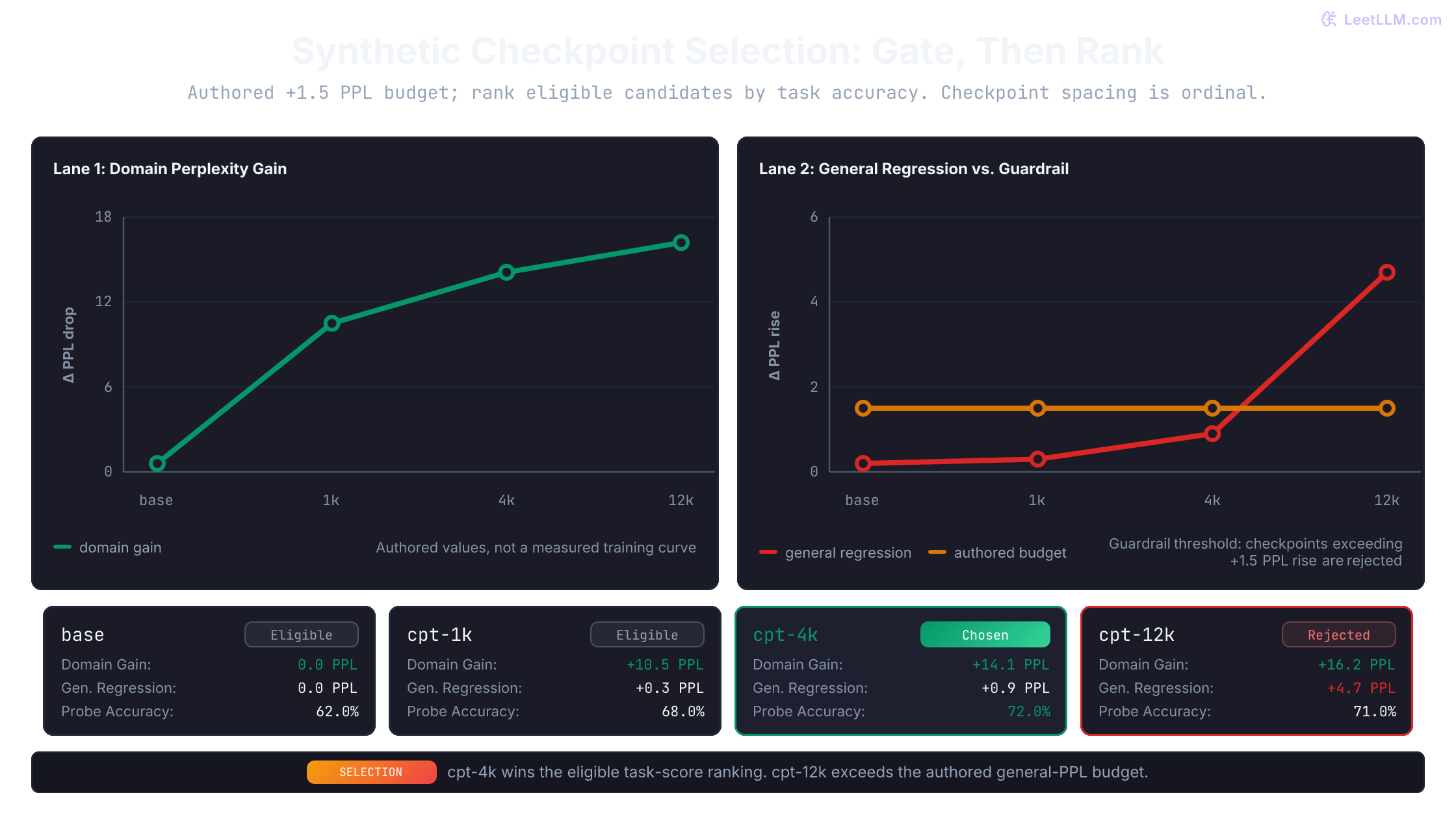
cpt-12k has the best domain perplexity but exceeds the allowed general-regression budget. cpt-4k passes the gate and has the best downstream probe accuracy among survivors. Which checkpoint wins?
Answer
Choose cpt-4k. General regression is a hard gate, so cpt-12k is ineligible. Among eligible checkpoints, downstream probe accuracy ranks first and domain perplexity only breaks ties.
Stopping rules
Because continued pretraining keeps the causal language modeling objective, runs can feel deceptively safe. They aren't safe by default. You stop when downstream probe accuracy plateaus, when domain validation loss flattens, or when general regressions approach your safety threshold.
Unused documents and a tiny loss decrease aren't sufficient reasons to keep spending compute. Set a patience window, minimum worthwhile gain, and regression limits, then consider metric uncertainty and evaluation cost. Two flat checkpoints or a 0.2-percentage-point change aren't universal stopping rules. For 500 binary task cases, one changed outcome already moves accuracy by 0.2 percentage points. Reusing the same cases for many selections can overfit the evaluation; confirm the chosen recipe on a reserved test set.
At a selected checkpoint, save weights, tokenizer, config, corpus manifest, and evaluation protocol. For exact continuation also save optimizer/scheduler state, RNG states, and loader cursors. Test the intended final assistant after its actual post-training recipe before promotion.
Where it fits relative to LoRA and SFT
Compare the choices by asking what you want to change.
| Goal | Candidate approach |
|---|---|
| Inject fresh or citable facts without retraining | RAG |
| Teach new domain language patterns | continued pretraining |
| Teach chat or task format | SFT |
| Run a behavior update without full-weight training | SFT with LoRA / QLoRA adapters |
| Choose between multiple acceptable responses | DPO or RLHF |
LoRA and QLoRA are parameter-efficient implementation choices; QLoRA also stores the frozen base model in quantized form.[11] They don't determine what supervision teaches. An adapter can be trained with a next-token domain-text objective or with prompt-response SFT. First choose objective from the failure mode, then choose full-weight or parameter-efficient training from budget and deployment constraints.
A training stack can run from base model to continued pretraining on a domain corpus, then SFT on curated prompt-response data, with preference optimization if needed. Not every product needs every stage. Compare stages against the failure you observe. Code Llama's Instruct variants are one shipped example: code pretraining followed by instruction tuning.[5] Llama 3's code expert combined continued pretraining with SFT and DPO, then helped produce annotations and synthetic data for the main model.[12]
Common pitfalls
Using continued pretraining to fix assistant tone
Poor formatting motivates an SFT comparison. Also inspect the chat template, decoding, and supplied instructions; a malformed interface can make capable weights appear unhelpful.
Over-specializing on one corpus
If domain completions improve while the model becomes narrow or brittle elsewhere, suspect a missing replay mixture or too many adaptation steps. Keep a general-text regression lane and stop earlier.
Skipping the downstream check
If domain perplexity improves but the final task model barely benefits, the adaptation run optimized text fit that didn't transfer to the product task. Probe the adapted checkpoint with a small downstream SFT instead of judging only by perplexity.