Personalize this lesson
Adapt explanations and teaching visuals to your background and preferred voice.
At noon, a job-risk service is responding in 40 milliseconds and returning scores. Its uptime and latency dashboards are bright green. One request, however, contains a three-hour-old queue snapshot. Another job's outcome won't be known until tomorrow. Endpoint uptime answers neither whether today's inputs are usable nor whether yesterday's predictions helped.
Two useful monitoring clocks are:
- The Fast Request Clock: Synchronous, pre-scoring input health checks that can reject or quarantine an inference payload immediately.
- The Slow Outcome Clock: Asynchronous, post-maturity evaluation loops that must wait for the label delay before calculating precision, recall, or business error cost.
We'll simulate both for a model that flags batch jobs likely to miss deadlines, then propose promotion and rollback outcomes from authored gate results. The standard-library Python cells share one session. Scores, cohort counts, and latency values are fixtures; no model is fitted, request routed, notification sent, or deployment changed.
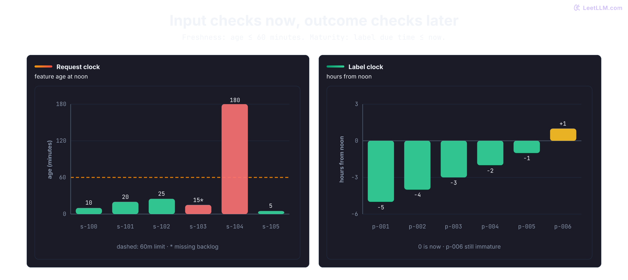
s-104 is 180 minutes old and blocks immediately; s-103 is fresh at 15 minutes but lacks queue_backlog, so it blocks on completeness. The slow label clock (right) measures prediction maturity in hours from noon. Five predictions are mature; p-006 at +1h remains immature and stays out of the quality cohort.Start with a served release and feature traces
Before asking whether a prediction is right, capture what it saw. We'll score each live job for service-level agreement (SLA)-miss risk. High scores enter operational review. Each request carries two model inputs:
| Feature | Meaning | Why it can fail |
|---|---|---|
queue_backlog | jobs waiting in the runner pool | upstream feed drops or changes measurement units |
hours_since_last_heartbeat | elapsed time since the latest scheduler heartbeat | stale worker snapshot or timestamp parsing error |
A 30-hour-old heartbeat can be a valid risk signal in a freshly computed feature. That's different from a feature snapshot that hasn't been refreshed for three hours. Monitor the age of the measurement separately from the value it measures.
Store a feature trace with each prediction: values, timestamps, and feature-contract versions. Replay also needs preserved model bytes, transforms, and input revisions; mutable version names alone aren't enough. Restrict sensitive traces and their retention to the investigation's needs.
Build six incoming requests against deployed release job-risk-v3. Two rows contain failures that should be caught before delayed SLA labels exist. The fixture scores stand in for model outputs; they must not be used for blocked requests.
from datetime import datetime, timedelta, timezone
from hashlib import sha256
from json import dumps
from math import isclose, isfinite, log

now = datetime(2026, 2, 4, 12, 0, tzinfo=timezone.utc)
deployed = {
    "model": "job-risk-v3",
    "feature_contract": "features-v3",
    "threshold": 0.50,
}
requests = [
    {"job_id": "s-100", "runner_pool": "fc-a", "queue_backlog": 18, "hours_since_last_heartbeat": 2, "feature_as_of": now - timedelta(minutes=10), "risk_score": 0.18},
    {"job_id": "s-101", "runner_pool": "fc-a", "queue_backlog": 27, "hours_since_last_heartbeat": 8, "feature_as_of": now - timedelta(minutes=20), "risk_score": 0.44},
    {"job_id": "s-102", "runner_pool": "fc-b", "queue_backlog": 35, "hours_since_last_heartbeat": 20, "feature_as_of": now - timedelta(minutes=25), "risk_score": 0.76},
    {"job_id": "s-103", "runner_pool": "fc-b", "queue_backlog": None, "hours_since_last_heartbeat": 26, "feature_as_of": now - timedelta(minutes=15), "risk_score": None},
    {"job_id": "s-104", "runner_pool": "fc-a", "queue_backlog": 22, "hours_since_last_heartbeat": 6, "feature_as_of": now - timedelta(minutes=180), "risk_score": 0.52},
    {"job_id": "s-105", "runner_pool": "fc-b", "queue_backlog": 40, "hours_since_last_heartbeat": 30, "feature_as_of": now - timedelta(minutes=5), "risk_score": 0.91},
]
feature_traces = [
    {
        **request,
        "model": deployed["model"],
        "feature_contract": deployed["feature_contract"],
    }
    for request in requests
]

print("deployed:", deployed["model"])
print("feature contract:", deployed["feature_contract"])
print("feature traces:", len(feature_traces))
print("label status: pending")deployed: job-risk-v3
feature contract: features-v3
feature traces: 6
label status: pendingAt request time, you don't know which jobs will miss their SLA. You can still answer a narrower, urgent question: do required inputs exist, and are their timestamps fresh enough to trust?
Each trace associates the request with model and contract names. The next function checks the supplied values before labels arrive. It doesn't verify the deployed transform, per-feature lineage, or upstream progress: a newly stamped snapshot can still contain old source data.
Block invalid inputs before waiting for labels
Which rows meet the scoring contract? s-103 has a recent snapshot but no backlog value. s-104 has a value but a snapshot from three hours ago. Both should stop before the label clock can tell us what happened.
Pre-label health auditing guards the model across three synchronous dimensions:
- Feature Completeness: Detect sudden spikes in null or missing values. When upstream data extractors fail, missing fields often manifest as silent zeroes or
Nonevalues. - Schema Integrity: Validate data types and domain constraints. Required features must be finite, nonnegative numbers; backlog must be an integer.
- Freshness Lag: Measure the elapsed time between the feature snapshot timestamp (
feature_as_of) and the current scoring timestamp. Our feature freshness contract requires snapshots between zero and 60 minutes old, inclusive. Future timestamps are invalid; a system tolerating clock skew must declare that tolerance explicitly.
An invariant is a declared condition the system must preserve. Check completeness, domain validity, and freshness. These checks enforce this contract; passing them doesn't prove an input is correct or a score is safe for every use. Define a fallback for blocked requests rather than silently treating them as low risk.
required_features = ["queue_backlog", "hours_since_last_heartbeat"]
max_feature_age_minutes = 60

def request_health(row):
    reasons = []
    for name in required_features:
        value = row.get(name)
        if value is None:
            reasons.append("missing=" + name)
        elif type(value) not in (int, float) or not isfinite(value) or value < 0:
            reasons.append("invalid=" + name)
        elif name == "queue_backlog" and value != int(value):
            reasons.append("noninteger=" + name)
    snapshot = row.get("feature_as_of")
    if not isinstance(snapshot, datetime) or snapshot.utcoffset() is None:
        reasons.append("invalid=feature_as_of")
    else:
        feature_age = (now - snapshot).total_seconds() / 60
        if feature_age < 0:
            reasons.append("future=feature_as_of")
        elif feature_age > max_feature_age_minutes:
            reasons.append(f"stale={feature_age:g}m")
    return reasons

healthy_requests = []
for row in feature_traces:
    reasons = request_health(row)
    if reasons:
        print(row["job_id"], "-> block", ";".join(reasons))
    else:
        healthy_requests.append(row)
        print(row["job_id"], "-> score")

print("scored:", len(healthy_requests))
print("blocked:", len(feature_traces) - len(healthy_requests))s-100 -> score
s-101 -> score
s-102 -> score
s-103 -> block missing=queue_backlog
s-104 -> block stale=180m
s-105 -> score
scored: 4
blocked: 2s-103 fails completeness: its snapshot is only 15 minutes old, but queue_backlog is absent. s-104 fails freshness: its value exists, but its snapshot is 180 minutes old. Neither failure requires an outcome label to detect. This function checks individual requests; production monitoring also needs aggregate failure rates and source-progress checks.
Sculley et al. describe unstable data dependencies, input-data tests, live monitoring, prediction-bias checks, and alerts from upstream feature producers as production concerns.[1] A model's serving contract therefore has to watch the data systems around its weights, not only the endpoint process.
Why block s-104 before its SLA label arrives?
Answer
The three-hour-old feature snapshot violates this request-time contract. A future label may measure outcome quality, but doesn't waive the freshness requirement. Freshness alone also wouldn't establish correctness.
Measure drift without calling it failure
Passing input checks doesn't mean traffic resembles training. For the next comparison, expand from the six-request trace to two separate 100-request windows, using only requests that passed the same contract.
Data drift means an input distribution changed over time. Distribution checks give a signal before labels arrive, as Klaise et al. discuss.[2] A shift tells you where to look; it doesn't prove accuracy fell.
Compare the historical and current distributions for hours_since_last_heartbeat:
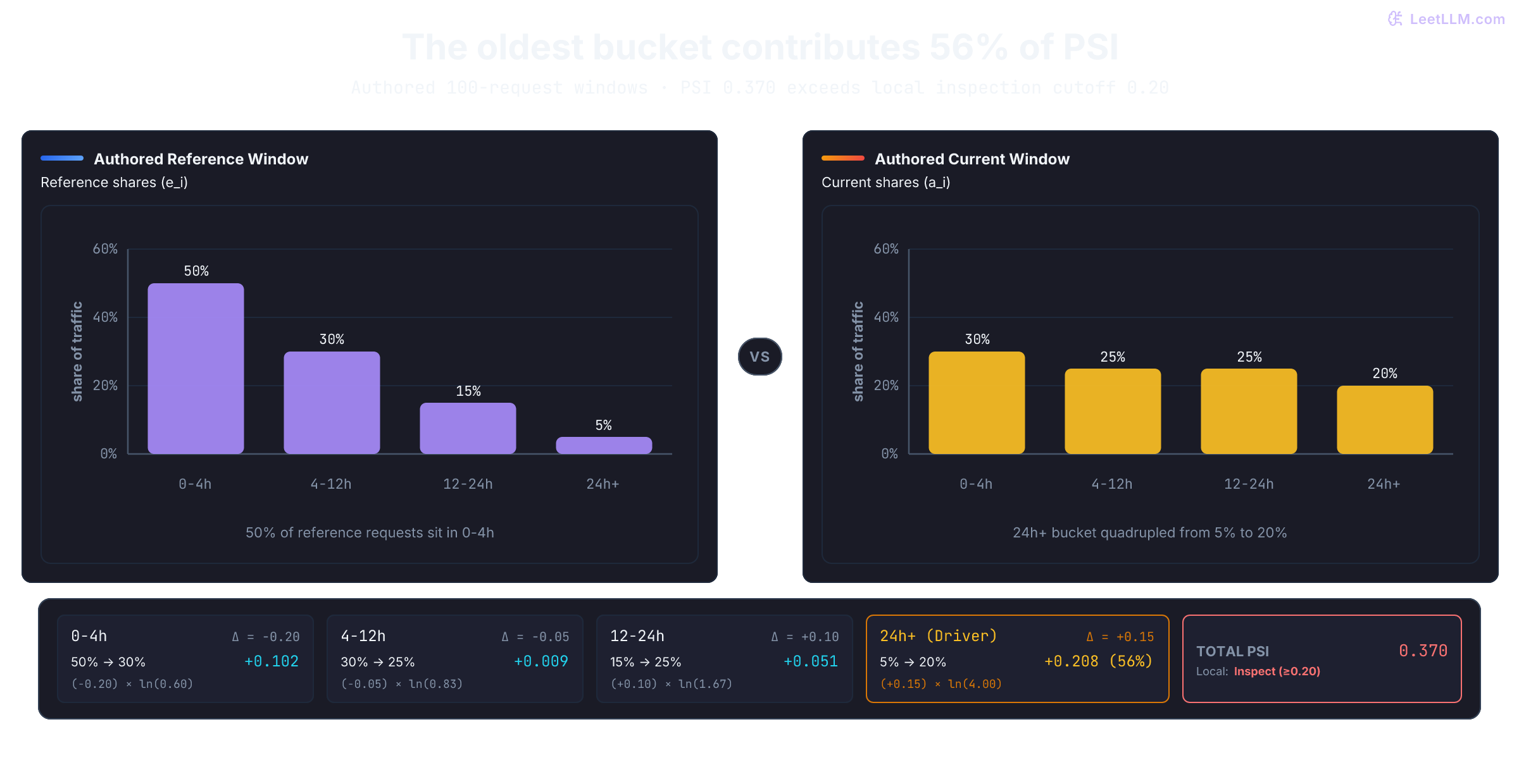
0.370, above the lab's 0.20 inspection cutoff. The 24h+ contribution is 0.208, about 56% of the total. Neither number establishes model-quality loss.The live window has more old heartbeats. A scheduler outage is one hypothesis. A holiday or a different runner-pool mix could create the same shape, so the histogram narrows the investigation without naming its cause.
Deriving the Population Stability Index
Compress the bucket pairs into the population stability index (PSI). With these normalized positive bin shares and natural logarithms, its formula equals Jeffreys divergence, the sum of both KL directions. This identity isn't a claim about the historical origin of PSI.
The KL divergence from current distribution to reference is:
Because KL divergence is asymmetric, comparing to yields a different quantity:
Summing both directions gives the symmetric divergence:
Here is the historical baseline share for bucket , and is its current live share. Notice that and always share the same sign: when , both terms are positive; when , both terms are negative. Their product is nonnegative, and is zero when the shares match.
The often-repeated 0.10/0.25 bands are historical rules of thumb, not universal standards or statistical significance levels. Sampling variation, sample size, bin count, dependence, and business relevance matter. A recent primary study discusses these limitations.[3] Our 0.20 threshold is an authored inspection policy, not a p-value, proof of failure, or automatic retraining trigger.
Use fixed bucket boundaries: 0-4h means , 4-12h means , and so on. Changing boundaries between windows would compare different events. PSI also loses changes within a bucket and relationships between features; two unchanged marginal histograms can hide a changed joint distribution.
Empty buckets need a declared policy. Below, an empty bucket in both windows contributes zero, but positive mass opposite zero gives infinite PSI. Optional additive smoothing adds the same pseudocount to every bucket before normalizing. It makes the result finite but changes the diagnostic, especially for small windows. Don't silently clip shares without renormalizing.
Work each term by hand across our four buckets:
0-4h:4-12h:12-24h:24h+:
Summing all four terms gives . The 24h+ bucket quadrupled from to and single-handedly drove over 56% of the total divergence. Our local policy investigates shifts at ; let's confirm the calculation in code.
bucket_names = ["0-4h", "4-12h", "12-24h", "24h+"]
reference_counts = [50, 30, 15, 5]
current_counts = [30, 25, 25, 20]

def normalize(counts, pseudocount=0.0):
    if not counts or any(not isfinite(x) or x < 0 for x in counts):
        raise ValueError("counts must be nonempty, finite, and nonnegative")
    if not isfinite(pseudocount) or pseudocount < 0 or sum(counts) == 0:
        raise ValueError("need observed data and a finite nonnegative pseudocount")
    adjusted = [count + pseudocount for count in counts]
    total = sum(adjusted)
    if not isfinite(total):
        raise ValueError("count total overflowed")
    return [count / total for count in adjusted]

def population_stability_index(reference, current):
    if len(reference) != len(current) or not reference:
        raise ValueError("bucket vectors must have the same nonzero length")
    for shares in (reference, current):
        if any(not isfinite(x) or x < 0 for x in shares) or not isclose(sum(shares), 1.0):
            raise ValueError("shares must be finite, nonnegative, and sum to one")
    terms = []
    for expected, actual in zip(reference, current):
        if expected == actual == 0:
            continue
        if expected == 0 or actual == 0:
            return float("inf")
        terms.append((actual - expected) * (log(actual) - log(expected)))
    return sum(terms)

reference = normalize(reference_counts)
current = normalize(current_counts)
psi = population_stability_index(reference, current)
investigate_at = 0.20

for name, before, after in zip(bucket_names, reference, current):
    print(f"{name}: reference={before:.2f} current={after:.2f} delta={after - before:+.2f}")
print("PSI:", round(psi, 3))
print("local action:", "inspect shift" if psi >= investigate_at else "continue")0-4h: reference=0.50 current=0.30 delta=-0.20
4-12h: reference=0.30 current=0.25 delta=-0.05
12-24h: reference=0.15 current=0.25 delta=+0.10
24h+: reference=0.05 current=0.20 delta=+0.15
PSI: 0.37
local action: inspect shiftThe code confirms 0.37, above the local 0.20 cutoff. Inspect source and traffic context; retraining isn't automatically the first fix. Repeating checks across many features and windows also needs a declared alert-volume and false-alarm policy.
Why shouldn't the 0.37 PSI result automatically start retraining?
Answer
PSI only reports a distribution change. Inspect source-data health, business context, and delayed outcomes first. Retraining on corrupted inputs can produce a newer broken model.
Continuous Drift Metrics: KS-Test and Wasserstein Distance
Unbinned one-dimensional distributions offer other diagnostics:
-
Kolmogorov-Smirnov (KS) Test: The two-sample KS-test computes the maximum vertical discrepancy between two empirical cumulative distribution functions (ECDFs):
measures shape discrepancy without bins. A standard p-value assumes independent samples from continuous distributions.[4] Counts, ties, repeated jobs, and serial dependence can undermine that calibration. Large independent samples can detect practically tiny differences; no universal sample-size or p-value boundary determines usefulness. Pair an appropriate test with effect size and operational impact.
-
Wasserstein Distance (Earth Mover's Distance): The 1D first Wasserstein distance measures the minimum cost (mass times distance) needed to reshape one probability distribution into another:
are CDFs, including those of discrete empirical distributions. has the feature's units when first moments are finite.[5] It describes the average transport distance under an optimal coupling, not a mean shift or movement of the same requests. Tail behavior, sampling error, dependence, and feature scaling still matter.
| Metric | Data Type | Binning Required? | Output Scale | Key Strength | Main Limitation |
|---|---|---|---|---|---|
| PSI | Categories or binned values | Fixed categories/bins | Dimensionless | Clear per-bin contributions | Binning, zero mass, sampling, and heuristic cutoffs |
| KS | 1D samples | No | ; optional p-value | Largest CDF discrepancy | Test assumptions; significance needn't imply impact |
| Wasserstein-1 | 1D distributions with finite first moments | No | Original feature units | Optimal transport interpretation | Tail sensitivity, scale, and local thresholds |
Two counterexamples help interpret the formulas. First, symmetric PSI doesn't satisfy the triangle inequality required of a metric. Second, two distributions can share a mean but have positive Wasserstein distance:
a, b, c = ([0.1, 0.9], [0.2, 0.8], [0.3, 0.7])
direct_psi = population_stability_index(a, c)
via_b_psi = population_stability_index(a, b) + population_stability_index(b, c)
print("direct PSI:", round(direct_psi, 3))
print("PSI via middle distribution:", round(via_b_psi, 3))
print("triangle inequality violated:", direct_psi > via_b_psi)

before_hours, after_hours = [0, 4], [2, 2]
# Equal sample sizes and weights: sorted pairing is optimal in one dimension.
w1_hours = sum(abs(x - y) for x, y in zip(sorted(before_hours), sorted(after_hours))) / 2
print("means:", sum(before_hours) / 2, sum(after_hours) / 2)
print("Wasserstein-1 hours:", w1_hours)direct PSI: 0.27
PSI via middle distribution: 0.135
triangle inequality violated: True
means: 2.0 2.0
Wasserstein-1 hours: 2.0The Drift Taxonomy: Covariate Shift, Concept Drift, and Label Drift
To isolate what actually moved, factor the joint data-generation distribution using Bayes' rule:
These terms describe distinct conditions, not mutually exclusive or exhaustive buckets:
- Covariate Shift (): The feature distribution changes while the underlying relationship remains invariant. For example, during a weekend batch surge, traffic shifts toward older scheduler heartbeats, but an 18-hour heartbeat carries the exact same probability of missing an SLA as it did during weekday training.
- Concept Drift (): The conditional relationship between inputs and targets changes. The real world changed: identical feature values now map to different outcome distributions. For example, infrastructure engineers deploy faster CPUs, so runners handle a queue backlog of 35 in minutes rather than hours. High backlog no longer implies an SLA miss.
- Label shift / prior probability shift: changes while remains fixed.[6] That invariance is a strong assumption, not something an increased miss rate proves. A cooling failure can also change features and their conditional relationships, so it isn't automatically pure label shift.
| Change | What moved | Early evidence | First response |
|---|---|---|---|
| Input distribution change | ; unchanged isn't yet established | feature PSI, KS, Wasserstein | inspect upstream data and traffic mix; evaluate later outcomes |
| Concept drift | (relationship) | persistent prediction errors within matched slices after checking labels | audit feature relevance and retrain on recent frozen snapshots |
| Outcome-rate change | ; pure label shift additionally requires fixed | mature outcome rates | inspect mix, labels, interventions, and conditional relationships |
For example, suppose two runner pools have unchanged miss rates of 10% and 40%. Moving their traffic mix from 50/50 to 80/20 lowers the overall miss rate from 25% to 16%, without changing either within-pool relationship. Base rates and aggregate quality can move just because the population changed. Conversely, can't change if both and remain fixed.
Score distributions give you another early signal before labels arrive. If raw risk scores shift while monitored feature histograms look stable, inspect the model version, serving configuration, transforms, and unmonitored feature relationships. A changed decision threshold changes review decisions, not the model's raw scores.
Reproduce training-serving skew
The same raw row should produce the same feature in both paths. Training-serving skew appears when production computes an input differently from training. Here, training divides backlog by staffed runner-pool capacity, while a serving change divides by a fixed 100.
Probe the same raw row through both transformations. Before reading the result, predict whether 20 / 50 can match 20 / 100.
probe = {"queue_backlog": 20, "staffed_capacity": 50}

def training_transform(row):
    return row["queue_backlog"] / row["staffed_capacity"]

def buggy_serving_transform(row):
    return row["queue_backlog"] / 100

training_value = training_transform(probe)
serving_value = buggy_serving_transform(probe)
print("training backlog ratio:", training_value)
print("serving backlog ratio:", serving_value)
print("parity:", training_value == serving_value)training backlog ratio: 0.4
serving backlog ratio: 0.2
parity: FalseThe same runner pool becomes 0.4 in training and 0.2 online, so the parity probe fails. Retraining won't repair that denominator. Share the transform, validate positive capacity upstream, and test several capacities rather than only 100, where the bug would hide. Compare unrounded values; if different numerical implementations require tolerance, set it from the feature's precision contract.
Google Cloud's MLOps guidance pairs unit tests for feature-engineering logic with prediction-service tests, data validation, and a predictive-performance check before deployment.[7] Those gates test the path that turns raw data into a served score, not only the final model artifact.
Join delayed labels back to stored predictions
Request-time checks move fast because they don't need outcomes. Quality moves on a slower clock: an SLA-miss label may arrive only after the promised job window closes. Passing the input contract permits scoring; it isn't evidence that the score was useful.
The Anatomy of the Delayed Label Problem
Tracking ground truth requires distinguishing three timestamps for every inference event:
- Prediction Timestamp (): When the model computed the score.
- Event Timestamp (): When the job actually completed or missed its SLA.
- Label Ingestion Timestamp (): When the verified outcome landed in the data warehouse.
Let be the end of the cohort's prediction-time window. For a declared outcome definition with common horizon , all of its outcome windows have closed once:
Different jobs may have different due times, so our code checks each row's label_due_at. Window closure doesn't ensure label arrival, correctness, or finality. A fixed-horizon miss label also differs from an eventual completion label.
Early-label selection can bias quality: jobs that fail quickly may be labeled before longer successful jobs, or the reverse under another collection path. Define cohorts before inspecting outcomes and report coverage. If you deliberately evaluate early outcomes, use a suitable censoring/time-to-event method and name that different estimand.
Proxy Metrics While Waiting for Labels
When true labels take weeks to mature, monitor near-instant proxy metrics:
- Leading Operational Indicators: Early warning signals that correlate with downstream failure. If predicting job SLA misses, track intermediate queue wait times, worker dropout rates, or partial step execution latency.
- Score and decision telemetry: Track raw score distributions separately from the fraction crossing a decision threshold. A review-rate jump can result from a threshold change without any score change. Stable monitored input marginals don't rule out changed joint inputs, transforms, or model versions. Investigate the jump; neither “hallucinating risk” nor model failure follows before outcomes are checked.
What should happen to p-006, whose outcome is due in one hour? Store model ID, score, job ID, decision context, and the time when each outcome becomes mature. Later, join outcomes by immutable prediction ID and compute quality only on cohorts whose outcome windows have closed.
Report label coverage inside each mature cohort. A missing label in a mature cohort is a coverage gap, not an on-schedule outcome. The following archived predictions concern different jobs from the live feature trace. The label map is a snapshot of valid Boolean outcomes available at noon; a historical replay must filter labels by their arrival timestamp, not use tomorrow's warehouse state.
predictions = [
    {"prediction_id": "p-001", "job_id": "s-200", "risk_score": 0.15, "priority_job": False, "label_due_at": now - timedelta(hours=5)},
    {"prediction_id": "p-002", "job_id": "s-201", "risk_score": 0.32, "priority_job": False, "label_due_at": now - timedelta(hours=4)},
    {"prediction_id": "p-003", "job_id": "s-202", "risk_score": 0.68, "priority_job": True, "label_due_at": now - timedelta(hours=3)},
    {"prediction_id": "p-004", "job_id": "s-203", "risk_score": 0.78, "priority_job": False, "label_due_at": now - timedelta(hours=2)},
    {"prediction_id": "p-005", "job_id": "s-204", "risk_score": 0.91, "priority_job": True, "label_due_at": now - timedelta(hours=1)},
    {"prediction_id": "p-006", "job_id": "s-205", "risk_score": 0.84, "priority_job": True, "label_due_at": now + timedelta(hours=1)},
]
decision_policy = "missed-sla-threshold-050-v1"
predictions = [
    {
        **prediction,
        "model": deployed["model"],
        "feature_contract": deployed["feature_contract"],
        "decision_policy": decision_policy,
        "decision_threshold": deployed["threshold"],
    }
    for prediction in predictions
]
labels = {
    "p-001": False,
    "p-002": False,
    "p-003": True,
    "p-004": False,
    "p-005": True,
}

def join_mature_cohort(predictions, labels, as_of):
    ids = [row["prediction_id"] for row in predictions]
    if len(ids) != len(set(ids)):
        raise ValueError("prediction IDs must be unique")
    if any(type(value) is not bool for value in labels.values()):
        raise ValueError("labels must be Boolean outcomes, not unknown placeholders")
    mature = [row for row in predictions if row["label_due_at"] <= as_of]
    immature = [row for row in predictions if row["label_due_at"] > as_of]
    joined = [{**row, "missed_sla": labels[row["prediction_id"]]}
              for row in mature if row["prediction_id"] in labels]
    missing = [row["prediction_id"] for row in mature if row["prediction_id"] not in labels]
    coverage = len(joined) / len(mature) if mature else None
    return mature, immature, joined, missing, coverage

matured, immature, matured_labeled, missing_matured_labels, label_coverage = (
    join_mature_cohort(predictions, labels, now)
)

print("stored predictions:", len(predictions))
print("matured predictions:", len(matured))
print("joined matured labels:", len(matured_labeled))
print(f"matured label coverage: {label_coverage:.3f}")
print("missing matured labels:", missing_matured_labels)
print("immature predictions:", [row["prediction_id"] for row in immature])stored predictions: 6
matured predictions: 5
joined matured labels: 5
matured label coverage: 1.000
missing matured labels: []
immature predictions: ['p-006']Prediction p-006 stays out because its SLA outcome window hasn't closed. That's the right-hand clock in the opening figure: five bars sit before noon, while +1h remains immature. Label arrival doesn't define cohort maturity.
The five-row mature cohort has 100% label coverage. If one mature row were still unlabeled, expose the gap instead of assuming that the observed subset is representative. The simple quality policy below requires full coverage.
Keep the same five outcome windows but delay p-005's ingestion until 13:00. At noon, it is mature and missing, not immature:
label_events = [
    {"prediction_id": pid, "outcome": outcome,
     "ingested_at": now + timedelta(hours=1) if pid == "p-005" else now - timedelta(hours=1)}
    for pid, outcome in labels.items()
]
labels_known_at_noon = {
    event["prediction_id"]: event["outcome"]
    for event in label_events if event["ingested_at"] <= now
}
late_mature, _, _, late_missing, late_coverage = join_mature_cohort(
    predictions, labels_known_at_noon, now
)
print("mature rows:", len(late_mature))
print("known-label coverage:", late_coverage)
print("missing mature labels:", late_missing)mature rows: 5
known-label coverage: 0.8
missing mature labels: ['p-005']This event list assumes one correct record per prediction. Real corrections need immutable revisions and a declared as-of selection policy; filtering timestamps alone doesn't resolve conflicts or duplicates.
Why exclude p-006 from this quality cohort instead of counting it as an on-schedule job?
Answer
Its outcome window hasn't closed, so the prediction isn't mature. Replacing that unknown outcome with a negative label biases the report. Separately, missing labels for predictions that are already mature must reduce reported coverage and can block quality decisions.
Evaluate decisions and calibration
The mature cohort lets us reconstruct decisions. Scores at or above each prediction's stored threshold enter job-SLA review. Use that historical threshold, not today's configuration, or an audit could silently change yesterday's decisions. Require a nonempty, fully labeled cohort, then compute precision and recall, priority-job misses, and weighted error cost.
if not matured or missing_matured_labels:
    raise RuntimeError("quality metrics unavailable: empty or incompletely labeled cohort")

def predicted_missed_sla(row):
    return row["risk_score"] >= row["decision_threshold"]

true_positives = sum(predicted_missed_sla(row) and row["missed_sla"] for row in matured_labeled)
false_positives = sum(predicted_missed_sla(row) and not row["missed_sla"] for row in matured_labeled)
false_negatives = sum(not predicted_missed_sla(row) and row["missed_sla"] for row in matured_labeled)

def rate_or_none(numerator, denominator):
    return round(numerator / denominator, 3) if denominator else None

precision = rate_or_none(true_positives, true_positives + false_positives)
recall = rate_or_none(true_positives, true_positives + false_negatives)
missed_priority_job = sum(
    row["priority_job"] and row["missed_sla"] and not predicted_missed_sla(row)
    for row in matured_labeled
)
error_cost = false_positives * 2 + false_negatives * 10

print("precision:", precision)
print("recall:", recall)
print("missed priority jobs:", missed_priority_job)
print("error cost:", error_cost)precision: 0.667
recall: 1.0
missed priority jobs: 0
error cost: 2This error-cost proxy assigns 2 units to an unnecessary review and 10 to a missed SLA that wasn't flagged. It omits the cost of reviewing true positives, so it isn't total operating cost. These are local decision weights, not universal business values. If a rate's denominator is zero, report None: missing evidence isn't measured failure.
Good threshold decisions don't establish calibration. Guo et al. found that modern neural classifiers can be miscalibrated.[8] Calibration means that predictions assigned a score of 0.80 have an 80% positive-outcome frequency in the population being evaluated. Calibration across the whole population doesn't establish calibration in every runner pool or service tier. Compare average scores with observed job-SLA rates in two buckets:
score_buckets = [
    ("low", [row for row in matured_labeled if row["risk_score"] < 0.50]),
    ("high", [row for row in matured_labeled if row["risk_score"] >= 0.50]),
]

for name, rows_in_bucket in score_buckets:
    if not rows_in_bucket:
        print(f"{name}: n=0 average_score=None observed_missed_sla_rate=None")
        continue
    average_score = sum(row["risk_score"] for row in rows_in_bucket) / len(rows_in_bucket)
    observed_rate = sum(row["missed_sla"] for row in rows_in_bucket) / len(rows_in_bucket)
    print(
        f"{name}: n={len(rows_in_bucket)} "
        f"average_score={average_score:.3f} "
        f"observed_missed_sla_rate={observed_rate:.3f}"
)low: n=2 average_score=0.235 observed_missed_sla_rate=0.000
high: n=3 average_score=0.790 observed_missed_sla_rate=0.667Three high-score jobs yield an observed rate of two out of three; one extra positive would move it to three out of four. That sensitivity is why this gap isn't evidence enough to approve or reject calibration. Use larger mature windows, uncertainty estimates, and relevant slices such as runner pool and service tier. Also record interventions: if review prevents a predicted SLA miss, the eventual label describes the intervened outcome. Comparing it directly with an untreated-risk prediction can mislead.
Triage repair, inspection, and retraining separately
By now, three signals can disagree: the feature mix may have shifted, a parity probe may fail, and delayed quality may fall. They don't imply the same action:
| Evidence | First action |
|---|---|
| missing or stale online features | repair data path |
| parity probe fails | repair training-serving contract |
| distribution shifts | inspect source health and business context |
| delayed decision cost regresses on adequate, comparable evidence | investigate labels and interventions; consider a frozen-snapshot candidate |
Repairs take precedence over retraining. In this small policy, quality_ready means the declared mature cohort has sufficient coverage and sample size, and the regression has survived checks for label, population, and intervention changes. It's an input from an investigation, not something PSI can establish.
def triage(schema_failures, stale_features, parity_ok, psi, cost_regressed, quality_ready):
    actions = []
    if schema_failures or stale_features:
        actions.append("repair online data path")
    if not parity_ok:
        actions.append("repair training-serving parity")
    if psi >= investigate_at:
        actions.append("inspect distribution shift")
    if not quality_ready:
        actions.append("withhold quality decision")
    if not schema_failures and not stale_features and parity_ok and quality_ready and cost_regressed:
        actions.append("train frozen-snapshot candidate")
    return actions

print("dirty window:", triage(1, 1, False, psi, True, True))
print("clean changed window:", triage(0, 0, True, psi, True, True))
print("labels incomplete:", triage(0, 0, True, psi, True, False))dirty window: ['repair online data path', 'repair training-serving parity', 'inspect distribution shift']
clean changed window: ['inspect distribution shift', 'train frozen-snapshot candidate']
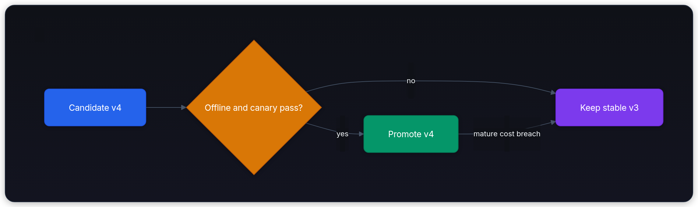
labels incomplete: ['inspect distribution shift', 'withhold quality decision']Continuous training produces candidates; it needn't overwrite production after every alert. Google Cloud describes several pipeline triggers and recommends tracking the previous model.[7] Separate the decision to run an experiment from the decision to expose its outputs to users:
Freeze an immutable candidate bundle
When clean evidence justifies new weights, freeze the snapshot, training pipeline, feature contract, decision policy, evaluation policy, and previous model pointer. The resulting candidate bundle is an immutable release proposal. Promotion moves an alias; it doesn't rewrite the bundle.
What must remain fixed if a later rollback needs to explain this candidate? Hash a manifest to identify its contents. A hash doesn't make referenced files immutable: production storage must preserve the exact data snapshot, model bytes, code, and contracts, with content digests or immutable revisions. This simulation hashes only the manifest and doesn't publish artifacts.
candidate_config = {
    "model": "job-risk-v4",
    "snapshot": "labels-through-2026-02-03",
    "training_pipeline": "job-risk-train-v4",
    "feature_contract": "features-v3",
    "decision_policy": decision_policy,
    "threshold": 0.50,
    "evaluation_policy": "job-risk-eval-v1",
    "previous_model": deployed["model"],
}
payload = dumps(candidate_config, sort_keys=True, separators=(",", ":"))
bundle_id = "job-risk-v4-" + sha256(payload.encode()).hexdigest()[:10]
candidate_bundle = {**candidate_config, "bundle_id": bundle_id}

print("candidate bundle:", candidate_bundle["bundle_id"])
print("rollback pointer:", candidate_bundle["previous_model"])candidate bundle: job-risk-v4-edde9c2176
rollback pointer: job-risk-v3The short bundle ID is a display label, not a collision-proof registry key. Keep the full digest in a real registry, and bind immutable artifact references rather than mutable names like latest. Google Cloud recommends lineage metadata and a previous-model pointer for rollback or comparison.[7]
Deployment strategies and canary health gates
Staged releases limit exposure while collecting evidence. Three common strategies answer different questions:
- Shadow traffic: Send a sample of live requests to the candidate while continuing to return the stable model's responses. Shadow predictions help inspect behavior and resource use, but mustn't trigger real review actions. Shared compute, queues, network traffic, and logging can still affect users; shadowing needs resource limits, data controls, and side-effect isolation.
- Canary routing: Assign a stable subset of jobs or users to the candidate, then increase exposure when declared checks pass. Choose an assignment unit that keeps related interactions together. A fast gate can request an abort, but telemetry delay, controller timing, and in-flight requests determine how quickly exposure stops. Shared resources can transmit effects beyond the assigned subset.
- Blue-green switching: Keep an active environment and a prepared replacement, then change the routing configuration after validation. Retaining the old environment can make reversal faster, but readiness, database and feature compatibility, routing propagation, and in-flight work still matter. No strategy promises a globally instantaneous switch or a fixed rollback time. Argo Rollouts provides pre- and post-promotion analysis for blue-green releases.[9]
Python's built-in string hash is salted separately for each process, so hash(job_id) % 100 isn't a stable routing rule across processes.[10] Use a declared hash algorithm, encoding, assignment key, and fixed experiment namespace. Here, SHA-256 assigns jobs to 100 buckets; selecting five buckets targets approximately 5% of jobs, not exactly 5% of requests:
def canary_bucket(job_id):
    key = ("job-risk-canary-v1:" + job_id).encode("utf-8")
    return int.from_bytes(sha256(key).digest()[:8], "big") % 100

def assigned_to_canary(job_id, percentage):
    if type(percentage) is not int or not 0 <= percentage <= 100:
        raise ValueError("percentage must be an integer from 0 to 100")
    return canary_bucket(job_id) < percentage

job_ids = [f"job-{i:04d}" for i in range(1000)]
at_five = {job_id for job_id in job_ids if assigned_to_canary(job_id, 5)}
at_twenty_five = {job_id for job_id in job_ids if assigned_to_canary(job_id, 25)}
print("jobs in 5 buckets:", len(at_five))
print("jobs in 25 buckets:", len(at_twenty_five))
print("same ID, same bucket:", canary_bucket("job-0000") == canary_bucket("job-0000"))
print("5-bucket group retained at 25:", at_five <= at_twenty_five)jobs in 5 buckets: 48
jobs in 25 buckets: 257
same ID, same bucket: True
5-bucket group retained at 25: TrueChanging the namespace reassigns jobs. Keep it fixed when increasing exposure in the same experiment. Jobs can make different numbers of requests, and this assignment alone doesn't establish a valid experiment or remove interference. The code computes membership; it doesn't send network traffic.
Use a separate held-out cohort to compare the candidates offline. The following synthetic confusion counts each total 1,000 predictions with 10 positive outcomes. Current v3 catches eight positives and makes 20 false alarms: its error cost is . Candidate v4 catches nine and makes 15 false alarms: . Express cost per 1,000 predictions so a later 500-row window can use the same units. The p95 latency values are also fixtures, not measured benchmarks.
def summarize_counts(tp, fp, fn, tn, priority_misses, latency_ms):
    counts = (tp, fp, fn, tn, priority_misses)
    if any(type(x) is not int or x < 0 for x in counts) or priority_misses > fn:
        raise ValueError("invalid confusion counts")
    n = tp + fp + fn + tn
    if not n or not isfinite(latency_ms) or latency_ms < 0:
        raise ValueError("need a nonempty cohort and valid latency")
    return {
        "n": n,
        "recall": tp / (tp + fn) if tp + fn else None,
        "priority_misses": priority_misses,
        "error_cost_per_1000": 1000 * (2 * fp + 10 * fn) / n,
        "p95_latency_ms": latency_ms,
    }

current_metrics = summarize_counts(8, 20, 2, 970, 1, 40)
candidate_metrics = summarize_counts(9, 15, 1, 975, 0, 42)
evaluation_cohort = {
    "maturity_cutoff": "2026-02-03T12:00:00Z",
    "matured_predictions": 1000,
    "joined_labels": 1000,
}
evaluation_cohort["label_coverage"] = (
    evaluation_cohort["joined_labels"] / evaluation_cohort["matured_predictions"]
    if evaluation_cohort["matured_predictions"] else None
)
offline_evaluation = {
    "policy": candidate_bundle["evaluation_policy"],
    "label_snapshot": candidate_bundle["snapshot"],
    "cohort": evaluation_cohort,
    "current": current_metrics,
    "candidate": candidate_metrics,
}
offline_gates = {
    "mature_label_coverage": evaluation_cohort["matured_predictions"] > 0 and evaluation_cohort["label_coverage"] == 1.0,
    "same_cohort_size": current_metrics["n"] == candidate_metrics["n"] == evaluation_cohort["joined_labels"],
    "recall": candidate_metrics["recall"] is not None and current_metrics["recall"] is not None and candidate_metrics["recall"] >= current_metrics["recall"],
    "priority_misses": candidate_metrics["priority_misses"] == 0,
    "error_cost": candidate_metrics["error_cost_per_1000"] <= current_metrics["error_cost_per_1000"],
    "latency_budget": candidate_metrics["p95_latency_ms"] <= 50,
}

for name, passed in offline_gates.items():
    print(f"{name}: {passed}")
print("offline gate:", all(offline_gates.values()))mature_label_coverage: True
same_cohort_size: True
recall: True
priority_misses: True
error_cost: True
latency_budget: True
offline gate: TrueAll fixture checks pass for this local policy. Matching cohort sizes alone doesn't prove matching records: a real evaluation must score both models on the same immutable prediction IDs and label snapshot. Ten positives also give weak evidence about recall; predeclare sample requirements and uncertainty checks for important slices. These checks illustrate gate logic, not statistical approval. Google Cloud recommends online validation before full deployment.[7]
The canary asks a different question from the offline cohort: does this candidate stay within declared operational budgets under production-shaped traffic? Gate it on fast signals such as service errors, latency, request count, and immediate review-queue pressure. Declare each measurement window and denominator. Here, all values are authored fixtures; queue load is queued review work divided by the local capacity budget. These checks don't replace delayed-label quality or establish safety for unmeasured behavior.
canary_metrics = {
    "requests": 500,
    "error_rate": 0.002,
    "p95_latency_ms": 44,
    "review_queue_load_ratio": 0.72,
}
canary_gates = {
    "enough_requests": canary_metrics["requests"] >= 500,
    "error_rate": canary_metrics["error_rate"] <= 0.005,
    "p95_latency_ms": canary_metrics["p95_latency_ms"] <= 50,
    "review_queue_load_ratio": canary_metrics["review_queue_load_ratio"] <= 0.80,
}
canary_evaluation = {
    "policy": "job-risk-canary-v1",
    "metrics": canary_metrics,
    "checks": canary_gates,
}

for name, passed in canary_gates.items():
    print(f"{name}: {passed}")
print("canary gate:", all(canary_gates.values()))enough_requests: True
error_rate: True
p95_latency_ms: True
review_queue_load_ratio: True
canary gate: TrueArgo Rollouts supports metric analysis and aborts; its blue-green post-promotion analysis can switch traffic back to the previous stable ReplicaSet.[9] Our simulation uses that control pattern without invoking a deployment tool. A request-count minimum alone isn't statistical confidence, and shared queues mean a canary's impact can extend beyond its own requests.
Simulate promotion and rehearse rollback
In a deployment, passing both gate sets can authorize an alias update while leaving the bundle fixed. Here, a function returns the proposed final alias without changing any router or registry. Simulate a slower delayed-label guardrail arriving after promotion. The cost threshold is evaluated only after the declared mature cohort reaches full label coverage; an incomplete cohort reports insufficient evidence instead of treating early labels as representative. Operational emergencies can require stopping exposure before labels arrive.
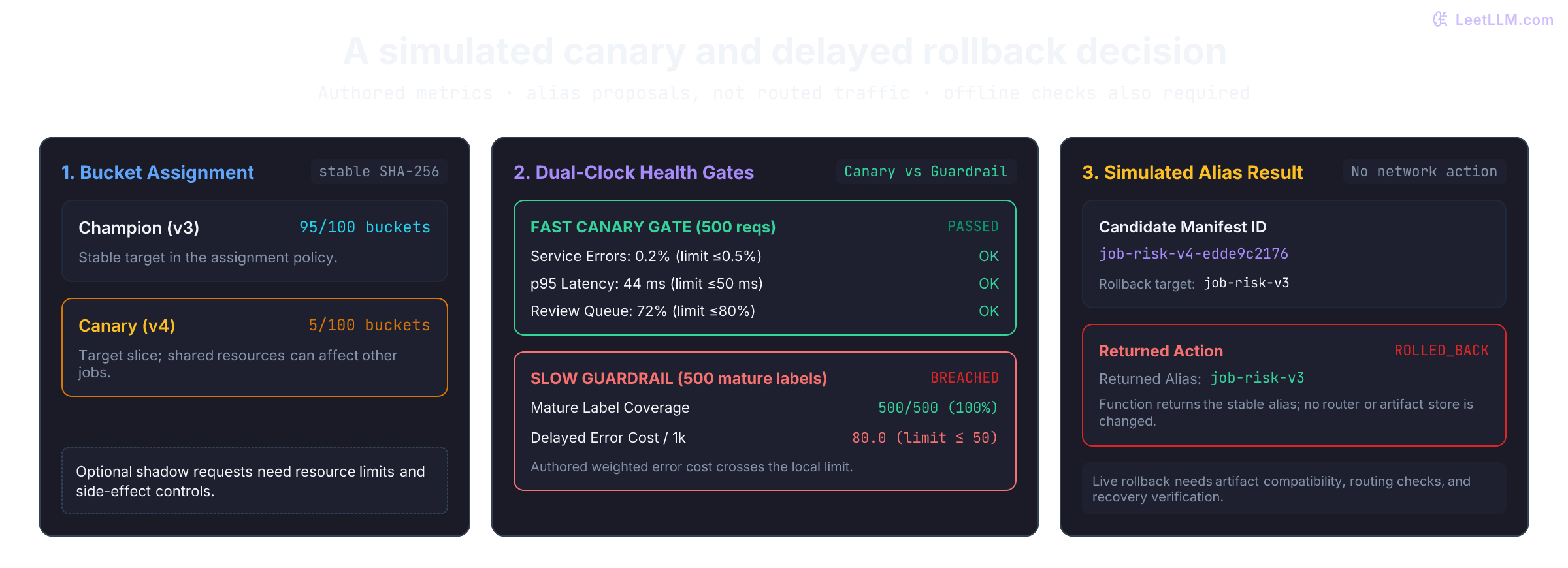
80 > 50), so the function returns job-risk-v3. This diagram illustrates policy decisions; it doesn't report a live rollout.def simulate_release(offline_ok, canary_ok, mature_count, joined_count, cost_per_1000):
stable = deployed["model"]
candidate = candidate_bundle["bundle_id"]
# No promotion means no post-promotion rollback can have occurred.
if not offline_ok or not canary_ok:
return {"action": "not_promoted", "alias": stable}
if any(type(n) is not int or n < 0 for n in (mature_count, joined_count)) or joined_count > mature_count:
raise ValueError("invalid label counts")
# Local policy: at least 500 mature rows, all labeled.
if mature_count < 500 or joined_count != mature_count:
return {"action": "insufficient_evidence", "alias": candidate}
if cost_per_1000 is None or not isfinite(cost_per_1000) or cost_per_1000 < 0:
return {"action": "invalid_metric", "alias": candidate}
rollback_limit = 50
if cost_per_1000 > rollback_limit:
return {"action": "rolled_back", "alias": stable,
"reason": f"error cost per 1000 {cost_per_1000:g} > {rollback_limit}"}
return {"action": "keep_candidate", "alias": candidate}
# 500 mature rows: two false negatives and ten false positives cost 40.
# In the same units as offline evaluation: 1000 * 40 / 500 = 80.
delayed_cost_per_1000 = 1000 * (2 * 10 + 10 * 2) / 500
receipt = simulate_release(all(offline_gates.values()), all(canary_gates.values()),
500, 500, delayed_cost_per_1000)
print("delayed error cost per 1000:", delayed_cost_per_1000)
print("release action:", receipt["action"])
print("final alias:", receipt["alias"])
print("reason:", receipt.get("reason"))
for name, args in [
("canary failed", (True, False, 500, 500, 80)),
("labels incomplete", (True, True, 500, 499, 80)),
("no mature rows", (True, True, 0, 0, None)),
("exact cost limit", (True, True, 500, 500, 50)),
]:
print(name + ":", simulate_release(*args)["action"])delayed error cost per 1000: 80.0
release action: rolled_back
final alias: job-risk-v3
reason: error cost per 1000 80 > 50
canary failed: not_promoted
labels incomplete: insufficient_evidence
no mature rows: insufficient_evidence
exact cost limit: keep_candidateThe main scenario returns a rollback decision: normalized cost 80 exceeds the local limit 50. At exactly 50, the strict > check returns keep_candidate. A failed canary returns not_promoted. Missing labels return the candidate alias with insufficient-evidence status. A production policy also needs a timeout and a decision about what to do if reliable evidence never arrives.
This function doesn't mutate deployment state. A real drill must resolve the stable artifact, check feature and schema compatibility, update routing only if the expected candidate is still active, and verify recovery. A conditional alias update can protect against conflicting controller actions; traffic propagation and in-flight work still need separate checks. Persist the cohort, thresholds, gate results, artifact identities, and reason with each decision. Restoring old weights doesn't undo reviews already triggered or repair an upstream data outage.
Does reverting to v3 guarantee cost falls below 50? No. Its earlier offline fixture already had cost 60, and neither offline fixture measures its performance in the later production window. The absolute-limit rule proposes a precautionary rollback, not a measured recovery. Check the restored model's contemporaneous outcomes and consider stopping or changing the review workflow if both models breach the budget.
When monitoring breaks
When an alert fires, identify which clock or contract broke before choosing a remedy:
| Symptom | Possible explanation | First check or action |
|---|---|---|
| Accuracy report arrives days after bad inputs hit production | only label metrics are monitored on slow loop | add schema, null-rate, and freshness alarms on fast request clock |
| Every drift alert immediately triggers automated retraining | covariate shift is confused with model failure | inspect data path, business context, and slice performance before retraining |
| Feature PSI is quiet but delayed error cost rises | concept drift, unmonitored feature shifts, or intervention feedback | compare matched slices, audit ground truth labels, and train snapshot candidates |
| Newly retrained model repeats wrong online predictions | serving transform differs from training pipeline | add automated parity probes before triggering training jobs |
| Dashboard looks pristine while labels are still arriving | metrics evaluate whichever labels arrived first | define mature cohorts, report label coverage, and block premature quality decisions |
| New model can't be rolled back cleanly | missing artifacts, incompatible state, or bundle and alias identities mixed up | preserve artifacts and contracts, protect alias updates, and verify recovery |
| Canary passes cleanly but delayed error cost later spikes | only fast telemetry was checked during rollout | maintain post-promotion guardrails and rehearse automated rollbacks regularly |