Personalize this lesson
Adapt explanations and teaching visuals to your background and preferred voice.
A developer searches a documentation portal for retry idempotency key. One matching document is a private postmortem draft, another is a deprecated v1 migration guide, and a third is an active, production-tested runbook buried on page two. Showing the private draft leaks confidential incident data. Missing the runbook leaves the developer stuck reading stale code.
Which documents may this developer see, which can we retrieve within the service's measured budget, and which survivor deserves the top slot? In single-item classification, a model scores each row independently: flag or pass. In ranking and recommendation systems, presentation order influences what developers see, click, and trust. A recommendation feed can use the same broad funnel without a typed query: user history, role, and session context supply request features.
Separate eligibility, retrieval, and ranking
Suppose your portal indexes one million documents. Running a costly joint query-document model on every row for every keystroke is usually impractical. A multi-stage design reduces candidate volume so later scorers can spend more compute per item. The counts below are an example design, not measurements from this portal. End-to-end latency also includes authorization, retrieval, networking, queueing, and rendering; measure it under representative load.
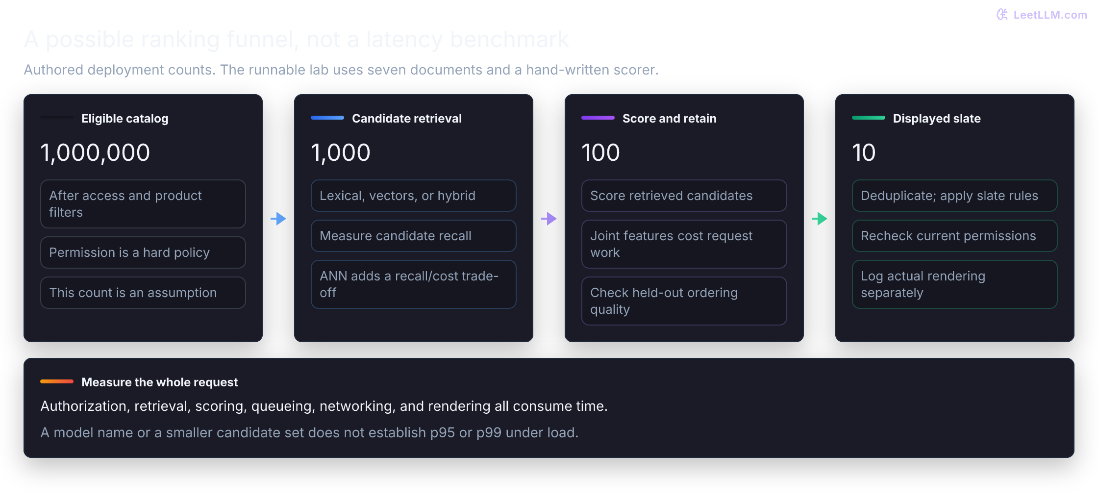
- Eligibility: Enforce access, tenancy, deletion, and product-specific freshness rules independently of learned scores. For this example design, suppose one million documents remain eligible. Filtering may be integrated with retrieval, and permissions must still be current at disclosure.
- Candidate retrieval (1,000,000 to 1,000): Retrieve a shortlist using lexical indexes, precomputed vectors, or their combination. Measure candidate recall and request cost: a relevant item dropped here can't be recovered by a ranker restricted to this set. Approximate vector search adds its own speed/recall trade-off.
- Scoring (1,000 to 100): Use query-document interactions, user affinities, and available context. DCN supplies a feature-interaction architecture; its loss is a separate choice. LambdaMART uses metric-weighted training updates. Neither guarantees the best final slate.
- Final slate (100 to 10): Apply deduplication and any declared source-diversity constraints, then recheck hard policies. Freshness boosts or sponsored placement are product choices, not universal stages. A constraint can lower unconstrained relevance metrics while satisfying the product contract.
A document that never enters the candidate set can't be rescued by a perfect ranker. For this lab, filter forbidden and stale documents before candidate generation. A search engine may integrate filtering into retrieval instead, but a high relevance score must never authorize disclosure. Recheck permissions at serving time if they can change after the index snapshot.
Build a seven-document fixture. Every score and judgment below is hand-assigned, not a measured model result. relevance is the evaluation target for this frozen query: 0 means no answer, 2 useful guidance, and 3 a direct answer. Grade 1 would mean marginally useful; none of these rows uses it. That label belongs in training or evaluation data, not among this request's serving features.
Before any scorer runs, inspect which rows survive the two hard filters. These Boolean fields stand in for request-specific policy decisions, not an implemented authorization service.
from hashlib import sha256
from json import dumps
from math import ceil, exp, log1p, log2

query = "retry idempotency key"
corpus = [
    {"id": "api-guide", "title": "retry idempotency API guide", "current": True, "permitted": True, "retrieval": 0.96, "query_fit": 0.98, "reliability": 0.88, "relevance": 3},
    {"id": "blog-post", "title": "general release blog", "current": True, "permitted": True, "retrieval": 0.91, "query_fit": 0.35, "reliability": 0.97, "relevance": 0},
    {"id": "legacy-changelog", "title": "legacy changelog", "current": True, "permitted": True, "retrieval": 0.90, "query_fit": 0.15, "reliability": 0.99, "relevance": 0},
    {"id": "retry-runbook", "title": "retry policy runbook", "current": True, "permitted": True, "retrieval": 0.84, "query_fit": 0.92, "reliability": 0.98, "relevance": 2},
    {"id": "sdk-example", "title": "idempotency SDK example", "current": True, "permitted": True, "retrieval": 0.80, "query_fit": 0.86, "reliability": 0.96, "relevance": 2},
    {"id": "private-draft", "title": "private retry incident draft", "current": True, "permitted": False, "retrieval": 0.99, "query_fit": 0.99, "reliability": 0.99, "relevance": 3},
    {"id": "stale-guide", "title": "stale retry migration guide", "current": False, "permitted": True, "retrieval": 0.95, "query_fit": 0.94, "reliability": 0.70, "relevance": 2},
]

print("corpus rows:", len(corpus))
print("query:", query)corpus rows: 7
query: retry idempotency keyThe corpus includes a private draft and a stale guide. Remove both before retrieval. A learned score can't override access policy.
eligible = [
    item
    for item in corpus
    if item["current"] and item["permitted"]
]
blocked = sorted(item["id"] for item in corpus if item not in eligible)

print("eligible:", [item["id"] for item in eligible])
print("blocked:", blocked)eligible: ['api-guide', 'blog-post', 'legacy-changelog', 'retry-runbook', 'sdk-example']
blocked: ['private-draft', 'stale-guide']Measure candidate recall before ordering quality
Candidate generation is the cheap retrieval stage. This lab uses a precomputed retrieval score so the contract between stages stays visible.
In Core Retrieval Algorithms, that stage was BM25, dense similarity, or a fused shortlist. The same contract appears here: recover the right documents first, then spend compute ordering them.
The judged relevant eligible documents are api-guide, retry-runbook, and sdk-example. Measure how many survive candidate generation. Predict what k=3 will miss before running the code.
relevant_ids = {
    item["id"]
    for item in eligible
    if item["relevance"] > 0
}

def candidates_at(limit):
    if not isinstance(limit, int) or limit < 0:
        raise ValueError("candidate limit must be a nonnegative integer")
    return sorted(
        eligible,
        key=lambda item: (-item["retrieval"], item["id"]),
    )[:limit]

def candidate_recall(items):
    if not relevant_ids:
        raise ValueError("recall needs at least one judged relevant eligible item")
    returned_ids = {item["id"] for item in items}
    return len(returned_ids & relevant_ids) / len(relevant_ids)

for limit in (3, 5):
    items = candidates_at(limit)
    print(
        f"k={limit} ids={[item['id'] for item in items]} "
        f"recall={candidate_recall(items):.3f}"
)k=3 ids=['api-guide', 'blog-post', 'legacy-changelog'] recall=0.333
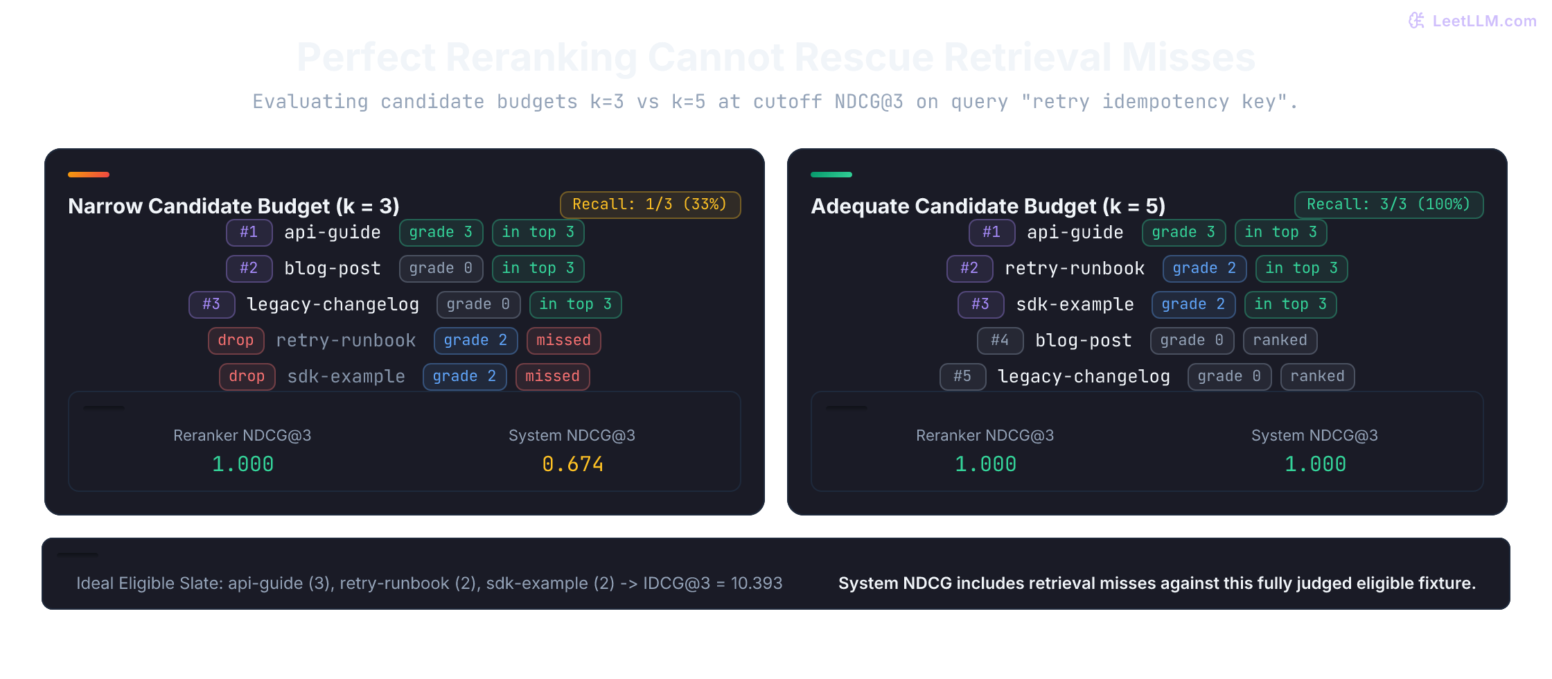
k=5 ids=['api-guide', 'blog-post', 'legacy-changelog', 'retry-runbook', 'sdk-example'] recall=1.000At k=3, retrieval keeps only one of three relevant eligible documents. This is a retrieval miss, not a ranking mistake: no downstream ranker can recover the missing runbook or SDK example.
Raising this candidate budget to 5 restores candidate recall before the expensive scorer runs. The next question is how to order those five survivors.
The relevant item never enters the top-100 candidate set. Can a more accurate reranker place it first?
Answer
No. Ranking can reorder only retrieved candidates. Fix candidate recall before interpreting downstream ordering metrics.
Rerank the surviving candidates
Keep five candidates. The first-stage retrieval order is fast but imprecise: blog-post and legacy-changelog sit near the top on retrieval alone, yet their query_fit stays low for the idempotency intent.
The scorer below is hand-written so each feature remains visible. query_fit stands for a richer query-document match signal, while reliability stands for source trust. Both are illustrative numbers on a 0-to-1 scale. Neither reads the offline relevance label, and the resulting score isn't a probability.
Before running it, predict whether the runbook moves above the generic blog.
candidates = candidates_at(5)

def rank_score(item):
    return 2.0 * item["query_fit"] + 0.6 * item["reliability"]

ranked = sorted(
    candidates,
    key=lambda item: (-rank_score(item), item["id"]),
)

print("retrieval order:", [item["id"] for item in candidates])
print("ranked order:", [item["id"] for item in ranked])
print("rank scores:", [(item["id"], round(rank_score(item), 3)) for item in ranked])retrieval order: ['api-guide', 'blog-post', 'legacy-changelog', 'retry-runbook', 'sdk-example']
ranked order: ['api-guide', 'retry-runbook', 'sdk-example', 'blog-post', 'legacy-changelog']
rank scores: [('api-guide', 2.488), ('retry-runbook', 2.428), ('sdk-example', 2.296), ('blog-post', 1.282), ('legacy-changelog', 0.894)]A learned scorer can estimate weights or nonlinear interactions from labeled examples. The request path stays the same: retrieve, score the bounded candidate set, then enforce final-slate constraints. Hold evaluation queries out of training and tuning; fitting these five rows would only memorize the demonstration.
The two orders of the same five documents are now ready to compare. Which one is actually better, and how much better is it?
Evaluate rank order with DCG, NDCG, MRR, and MAP
A classifier's accuracy doesn't care which mistakes you made first. A ranked list does. Putting the best document first is a much bigger win than sliding it from position 40 to position 39. To evaluate lists rigorously, ranking systems use position-discounted metrics.
Graded relevance and logarithmic discounting (DCG and NDCG)
The API guide has grade 3, while the runbook has grade 2. Exponential gain values those grades as , producing gains of 7 and 3. At rank 1 the full gain counts. This DCG convention uses the logarithmic discount to value earlier results more. That discount is a metric design choice, not a measured examination probability for this portal:
| Rank Position | Discount Denominator | Position Multiplier |
|---|---|---|
| 1 | 1.000 | |
| 2 | 0.631 | |
| 3 | 0.500 | |
| 4 | 0.431 | |
| 5 | 0.387 |
Discounted Cumulative Gain (DCG) sums those discounted gains across the top items:
Here is the judged relevance grade at position , counting from 1. This exponential-gain form rewards finding direct answers early.[1] Linear gain would use instead of ; both agree for binary labels , but exponential gain separates grade 3 answers from grade 2 guides.
Because DCG raw scores scale with the number of relevant documents for a query, comparing DCG across queries is noisy. Normalized DCG (NDCG) normalizes the metric by dividing by the Ideal DCG (IDCG), which is the DCG of the perfectly sorted list:
Work the retrieval order [3, 0, 0, 2, 2] by hand:
The ideal order of these five grades is [3, 2, 2, 0, 0]:
So retrieval-order NDCG@5 is . Build that ideal list from all candidate relevances before truncating. Otherwise a relevant candidate below the evaluated slate could disappear from the denominator.
Single-target and binary metrics: MRR and MAP
Different user journeys demand different evaluation metrics:
- Mean Reciprocal Rank (MRR): In navigational search or command-palette queries, the developer wants exactly one target (such as the login page or API root). MRR evaluates only the rank of the first relevant document:
Reciprocal discounting drops off much steeper than logarithmic discounting: rank 2 receives , rank 3 receives , and rank 5 drops to .
- Mean Average Precision (MAP@k): For informational queries with binary relevance labels (), MAP rewards putting all relevant documents near the top with high precision density:
where is precision at cutoff , and is the number of relevant documents in the declared judgment universe. This lab uses the capped denominator . Another convention retains even at a cutoff; it penalizes unretrieved relevant items more strongly. State the convention before comparing reports. Standard full-list AP assigns zero credit to relevant documents never retrieved.[1]
RR and AP describe one query. MRR and MAP average those values over a declared query set; similarly, average per-query NDCG with explicit query weights. Here RR treats only grade 3 as a target. AP treats grades 2 and above as relevant, while candidate recall accepts any positive grade: these latter choices coincide here, but would diverge after adding grade 1. An absent RR target gets zero; the code also assigns zero when no relevant item exists, a reporting convention to disclose.
def dcg(relevances):
    return sum(
        (2**relevance - 1) / log2(rank + 2)
        for rank, relevance in enumerate(relevances)
    )

def reranker_ndcg(items, limit):
    if not isinstance(limit, int) or limit <= 0:
        raise ValueError("evaluation cutoff must be a positive integer")
    if len({item["id"] for item in items}) != len(items):
        raise ValueError("duplicate document IDs would double-count gain")
    if any(item["relevance"] < 0 for item in items):
        raise ValueError("relevance grades must be nonnegative")
    relevances = [item["relevance"] for item in items[:limit]]
    ideal = sorted(
        (item["relevance"] for item in items),
        reverse=True,
    )[:limit]
    best = dcg(ideal)
    return dcg(relevances) / best if best else 0.0

def reciprocal_rank(items, target_grade=3):
    for rank, item in enumerate(items, start=1):
        if item["relevance"] >= target_grade:
            return 1.0 / rank
    return 0.0

def average_precision(items, threshold=2, limit=5):
    if not isinstance(limit, int) or isinstance(limit, bool) or limit <= 0:
        raise ValueError("evaluation cutoff must be a positive integer")
    evaluated = items[:limit]
    rel_count = 0
    precision_sum = 0.0
    for rank, item in enumerate(evaluated, start=1):
        if item["relevance"] >= threshold:
            rel_count += 1
            precision_sum += rel_count / rank
    total_rel = sum(1 for item in items if item["relevance"] >= threshold)
    return precision_sum / min(total_rel, limit) if total_rel else 0.0

print("retrieval-order ndcg@5:", f"{reranker_ndcg(candidates, 5):.3f}")
print("ranked-order ndcg@5:", f"{reranker_ndcg(ranked, 5):.3f}")
print("retrieval-order rr:", f"{reciprocal_rank(candidates):.3f}", "ap@5:", f"{average_precision(candidates):.3f}")
print("ranked-order rr:", f"{reciprocal_rank(ranked):.3f}", "ap@5:", f"{average_precision(ranked):.3f}")retrieval-order ndcg@5: 0.910
ranked-order ndcg@5: 1.000
retrieval-order rr: 1.000 ap@5: 0.700
ranked-order rr: 1.000 ap@5: 1.000Notice the contrast. Retrieval order already has RR 1.000: its grade-3 target is first. AP@5 is only 0.700 and NDCG@5 is 0.910 because irrelevant pages separate it from the runbook and SDK example. The hand-written scorer produces ideal ordering on this one fixture, giving both AP@5 and NDCG@5 1.000. That isn't measured generalization.
Check the denominator choice with two relevant documents and a one-slot display. Predict whether perfect top-slot precision gives the same AP under both conventions.
two_relevant = [{"id": "a", "relevance": 2}, {"id": "b", "relevance": 2}]
top_slot_precision_sum = 1.0
print("capped-denominator AP@1:", average_precision(two_relevant, limit=1))
print("full-R-denominator AP@1:", top_slot_precision_sum / len(two_relevant))capped-denominator AP@1: 1.0
full-R-denominator AP@1: 0.5Neither number is a coding error. They answer different questions. The existing helper counts relevant items in its supplied list, so it describes survivors; a whole-system AP denominator must come from the eligible judgment universe.
Reranker NDCG versus whole-system NDCG
This lab computes reranker NDCG over documents that survived retrieval. Candidate recall measures misses before ranking, while reranker NDCG measures ordering quality inside the bounded candidate set.
A whole-system evaluation also computes system NDCG against the eligible judged corpus so retrieval misses penalize the final score:
def system_ndcg(items, eligible_items, limit):
    reranker_ndcg(items, limit)
    reranker_ndcg(eligible_items, limit)
    judged = {item["id"]: item["relevance"] for item in eligible_items}
    if any(item["id"] not in judged or item["relevance"] != judged[item["id"]] for item in items):
        raise ValueError("results must use the eligible corpus and its frozen judgments")
    relevances = [item["relevance"] for item in items[:limit]]
    ideal = sorted(
        (item["relevance"] for item in eligible_items),
        reverse=True,
    )[:limit]
    best = dcg(ideal)
    return dcg(relevances) / best if best else 0.0

tight = candidates_at(3)
tight_ranked = sorted(
    tight,
    key=lambda item: (-rank_score(item), item["id"]),
)

print("k=3 survivors:", [item["id"] for item in tight_ranked])
print("k=3 grades:", [item["relevance"] for item in tight_ranked])
print("k=3 reranker ndcg:", f"{reranker_ndcg(tight_ranked, 3):.3f}")
print("k=3 system ndcg:", f"{system_ndcg(tight_ranked, eligible, 3):.3f}")k=3 survivors: ['api-guide', 'blog-post', 'legacy-changelog']
k=3 grades: [3, 0, 0]
k=3 reranker ndcg: 1.000
k=3 system ndcg: 0.674At k=3, the perfect reranker order among survivors still yields reranker NDCG 1.000, because the ideal list is built only from those three documents. System NDCG falls to 0.674 because the ideal top three from the eligible corpus is [3, 2, 2] and two relevant documents never entered the candidate slate.
All five eligible documents are judged here. In a real collection, incomplete judgments, changing eligibility, or a label policy that treats unjudged documents as irrelevant can change these denominators. Record the judgment version and coverage; a perfect judged score doesn't establish user value or authorization.
0.674.Why does normalized discounted cumulative gain (NDCG) penalize moving a relevant item from rank 1 to rank 10?
Answer
Discounted cumulative gain gives earlier positions more weight through a logarithmic discount. NDCG then divides by the ideal ordering, making the score comparable across queries with different relevance sets.
Two-tower retrieval and feature interaction networks
How can the first stage search a million documents without running the expensive ranker on each one? It moves heavy model compute out of the request path.
Candidate retrieval commonly uses a two-tower architecture.[2] One encoder (the query tower) maps the live query or session context to a vector . A separate encoder (the item tower) maps each document or item to a vector . The system computes similarity via dot product or cosine similarity.
Because the item tower doesn't depend on the current query, item vectors can be precomputed and searched with an ANN index, such as an HNSW graph or ScaNN. HNSW and ScaNN aren't themselves databases. Match the index's distance function to training: normalized dot product equals cosine similarity; unnormalized dot product also depends on vector magnitude. For dot-product retrieval, the request runs the query tower then approximate maximum-inner-product search. Index recall, freshness, and latency need measurement; no millisecond timings are established here.[3]
The vectors must be learned or supplied by a suitable pretrained encoder. A common retrieval objective makes an observed positive query/item pair score above sampled alternatives; those alternatives aren't verified dislikes. TFRS's example trains from positive pairs and evaluates against a candidate catalog.[3] Negative selection and repeated positives need care. Keep tower weights, normalization, item embeddings, and index version compatible; changing an encoder without rebuilding the corresponding vectors changes the scoring contract.
The cross-feature bottleneck
Two-tower similarity can serve as a final score when it meets the task's quality and cost needs. Its restriction is that each tower encodes its input independently; the final similarity couples them. A joint scorer can model richer early query-document interactions, at additional request cost.
An early cross-feature mixes query and item information before producing a score. A joint transformer is one example: query and document tokens can interact through attention. The document can still be cached or partly precomputed, but its complete joint representation generally changes with the query.
Restricting joint scoring to a shortlist reduces work. The resulting latency depends on token lengths, architecture, batches, hardware, and concurrency, rather than the shortlist size alone.
Deep and cross networks for heavy ranking
Deep & Cross Networks supply explicit feature interactions alongside a deep network. Distinguish the original DCN vector layer from DCN-v2's more expressive matrix layer.[4][5]
A possible input concatenates query, item, and context representations, . Categorical features can first be embedded. Cross and deep components can be parallel or stacked, not just parallel.[5]
- Cross network: The original vector-parameterized layer updates as:
Here . After such layers, the highest polynomial degree is at most . Terms share parameters; the layer doesn't freely assign an independent coefficient to every possible cross.[4]
The inner dot product is scalar, so this layer takes arithmetic. DCN-v2 instead uses elementwise multiplication :
A dense matrix layer costs . A factorization with rank costs roughly ; low-rank mixtures add their own expert and gating costs. These arithmetic counts don't guarantee a serving budget.[5]
- Deep Network: A standard multi-layer feed-forward network with non-linear activations (ReLU or GeLU) that captures implicit, non-linear interactions.
In a parallel binary click model, concatenate the components and use a sigmoid head with a declared click loss. Other heads and losses can predict grades or utilities. DCN architecture alone doesn't directly optimize NDCG or make click probabilities unbiased.[6]
from random import Random

rng = Random(42)
n_items = 1_000
dim = 16
candidate_budget = 5

def random_vector(size=dim):
    return [rng.gauss(0.0, 1.0) for _ in range(size)]

def dot(left, right):
    return sum(a * b for a, b in zip(left, right))

# Synthetic stand-ins for item-tower outputs, prepared before the query.
doc_embeddings = [random_vector() for _ in range(n_items)]
query_embedding = random_vector()

# Exact search stands in for an ANN lookup in this small lab.
retrieval_scores = [dot(doc, query_embedding) for doc in doc_embeddings]
candidate_ids = sorted(
    range(n_items),
    key=lambda item_id: (-retrieval_scores[item_id], item_id),
)[:candidate_budget]

def dcn_cross_layer(x_0, x_l, weight, bias):
    # x_{l+1} = x_0 * (x_l^T w) + b + x_l computed in O(D)
    scalar_proj = dot(x_l, weight)
    return [
        x0_i * scalar_proj + b_i + xl_i
        for x0_i, b_i, xl_i in zip(x_0, bias, x_l)
    ]

# Original DCN vector layer over concatenated query and item inputs.
w_cross = random_vector(2 * dim)
b_cross = random_vector(2 * dim)
cross_features = []
for item_id in candidate_ids:
    x_input = query_embedding + doc_embeddings[item_id]
    x_next = dcn_cross_layer(x_input, x_input, w_cross, b_cross)
    cross_features.append(x_next)

print("offline item vectors:", len(doc_embeddings))
print("live query vectors:", 1)
print("exact dot products on request:", len(retrieval_scores))
print("expensive candidates routed to DCN:", len(cross_features))
print("DCN output dimension:", len(cross_features[0]))offline item vectors: 1000
live query vectors: 1
exact dot products on request: 1000
expensive candidates routed to DCN: 5
DCN output dimension: 32These are random vectors and random cross weights, not trained encoders or measured relevance. Exact search still performs 1,000 dot products; the demonstration doesn't execute ANN or a latency benchmark. Five candidates receive a query-dependent original DCN vector layer. The item portion of that crossed representation must be recomputed for a changed query.
Check the two equations on a two-dimensional input. They differ in both parameterization and where the bias enters.
x0, xl = [2.0, 3.0], [5.0, 7.0]
vector_result = dcn_cross_layer(x0, xl, [1.0, 0.0], [0.5, 1.0])

def matrix_cross_layer(x_0, x_l, matrix, bias):
    return [
        base * (dot(row, x_l) + offset) + residual
        for base, row, offset, residual in zip(x_0, matrix, bias, x_l)
    ]

matrix_result = matrix_cross_layer(x0, xl, [[1.0, 0.0], [0.0, 1.0]], [0.5, 1.0])
print("original vector layer:", vector_result)
print("v2 matrix layer:", matrix_result)

probe_item = [1.0, 2.0]
probe_weight = [0.5, 0.25, 0.5, 0.25]
first = [0.0, 1.0] + probe_item
second = [1.0, 0.0] + probe_item
item_after_first = dcn_cross_layer(first, first, probe_weight, [0.0] * 4)[2:]
item_after_second = dcn_cross_layer(second, second, probe_weight, [0.0] * 4)[2:]
print("changed query changes crossed item:", item_after_first != item_after_second)original vector layer: [15.5, 23.0]
v2 matrix layer: [16.0, 31.0]
changed query changes crossed item: TrueNeither layer's output is a probability until a trained scoring head defines its meaning. These small helpers assume matching vector dimensions.
Evaluate a language-model reranker
A language model can also compare a retrieved group and return an order. RankGPT's 2023 study explored identifier permutations and sliding windows, and distilled those orders into smaller scorers. Those historical benchmark results aren't a current guarantee for your model or portal.[7] Compare a proposed reranker against lexical, two-tower, and simpler joint-scoring baselines on held-out queries, including cost and latency.
Give it the query and eligible document snippets with stable IDs. Ask for a permutation of those IDs, most useful first. Treat snippet instructions as untrusted document content. Keep access checks outside the model, and ensure any external processing is authorized before sending the snippets. A prompt alone doesn't enforce those boundaries.
Validate the output structurally, then evaluate its quality. The following response is hand-assigned, not returned by a model. Predict whether a valid permutation can nevertheless lower NDCG.
def validate_order(proposed_ids, candidate_items):
    expected = {item["id"] for item in candidate_items}
    if not isinstance(proposed_ids, list) or any(
        not isinstance(item_id, str) for item_id in proposed_ids
    ):
        raise ValueError("reranker output must be a list of document IDs")
    if len(proposed_ids) != len(expected) or set(proposed_ids) != expected:
        raise ValueError("reranker output must be an exact candidate permutation")
    by_id = {item["id"]: item for item in candidate_items}
    return [by_id[item_id] for item_id in proposed_ids]

# Candidate IDs are supplied separately for this independent code chain.
allowed_ids = ["api-guide", "retry-runbook", "sdk-example", "blog-post", "legacy-changelog"]
proposed_ids = ["retry-runbook", "api-guide", "sdk-example", "blog-post", "legacy-changelog"]
candidate_items = [{"id": item_id} for item_id in allowed_ids]
validated = validate_order(proposed_ids, candidate_items)
print("valid permutation:", len(validated) == len(candidate_items))
for invalid in [
    ["private-draft"] + allowed_ids[1:],
    [allowed_ids[0]] + allowed_ids[:-1],
]:
    try:
        validate_order(invalid, candidate_items)
    except ValueError:
        print("invalid candidate permutation rejected:", True)
    else:
raise AssertionError("invalid permutation was accepted")valid permutation: True
invalid candidate permutation rejected: True
invalid candidate permutation rejected: TrueThe accepted order swaps the grade-3 guide with the grade-2 runbook. On the original judgment fixture, NDCG@3 falls to about 0.858. Structural validation doesn't establish relevance or resistance to manipulation. Recheck current eligibility before display, and predeclare a safe fallback for timeout, invalid output, or an underfilled candidate list. Measure sensitivity to input order and adversarial snippets instead of assuming a generated explanation proves quality.
What changes for a recommendation feed?
Remove the typed query and keep the docs portal. A developer who has been reading retry guides might appreciate the SDK example next. The request-side tower encodes developer history and session context; the item tower still encodes each document independently.[3]
Two sources of evidence answer different questions:[8]
| Evidence | Docs-portal example | Missing-data problem |
|---|---|---|
| content-based | recommend a document whose topics resemble those the developer chose | a new developer has little preference history |
| collaborative | learn from developers who used overlapping documents | a new document has no interaction history |
An ID-only user/item embedding model is a matrix-factorization form of collaborative filtering. Towers that accept document text or metadata can also represent a newly indexed document before anyone clicks it.[3] That helps with missing interaction history, but doesn't prove the document is useful. Evaluate new users and new items separately instead of hiding them inside an average dominated by familiar ones.
Recommendations also need a time boundary: train on interactions available before a cutoff, then evaluate later outcomes. A future click must not enter a feature used to predict that same click.[3] An unseen item isn't automatically disliked; it may simply never have been exposed.
Learning to rank: pointwise, pairwise, and listwise
How do we train ranking models? Machine learning provides three distinct approaches:
| Family | Training target | Loss formulation | Limitation |
|---|---|---|---|
| pointwise | one item's grade, click, or utility | MSE or binary cross-entropy | A plain unweighted loss doesn't explicitly value rank position; context and weights can still be added |
| pairwise | a preferred item over another within the same query | RankNet logistic loss on | An unweighted pair with the same score gap has the same score derivative regardless of position |
| listwise | a query's ranked set or list distribution | ListNet/ListMLE-style objectives or differentiable metric surrogates | Requires a declared list/judgment universe; training can use sampled lists |
LambdaRank and LambdaMART use pairs weighted by a list metric. They are often grouped with metric-aware or listwise methods, but their update construction is pairwise, not a smooth derivative of NDCG.[9]
The pairwise loss (RankNet)
Pairwise methods such as RankNet train from preferences so a more relevant item scores above a less relevant one for the same query.[10]
Given a preferred document and a less relevant document , RankNet models the preference probability with a logistic function on their score difference :
The gradient with respect to score difference is . When the model gives both items equal scores (), and the gradient is .
Metric-weighted pairs: LambdaRank and LambdaMART
Consider two preferred/other pairs with equal score gaps. Plain RankNet gives them the same derivative with respect to that gap, even if one pair is near the top and another is deep in the list. Their feature/parameter gradients can still differ. A top-weighted metric such as NDCG values their position changes differently; user satisfaction isn't measured by that metric alone.
As a function of predicted scores with fixed judgments, NDCG is piecewise constant. It changes at ordering boundaries and has zero gradient away from them. A usual smooth gradient step therefore needs a surrogate or a constructed update.
LambdaRank constructs pairwise update signals weighted by a ranking utility. This isn't the exact derivative of the sorted NDCG score, nor a guarantee of finding its global maximum.[9]
For a preferred item and a lower-grade item , scale the logistic score derivative by , computed from their positions in the current ranked list. Here controls logistic steepness; our code uses :
For this scaled form, use ; the preceding RankNet example set .
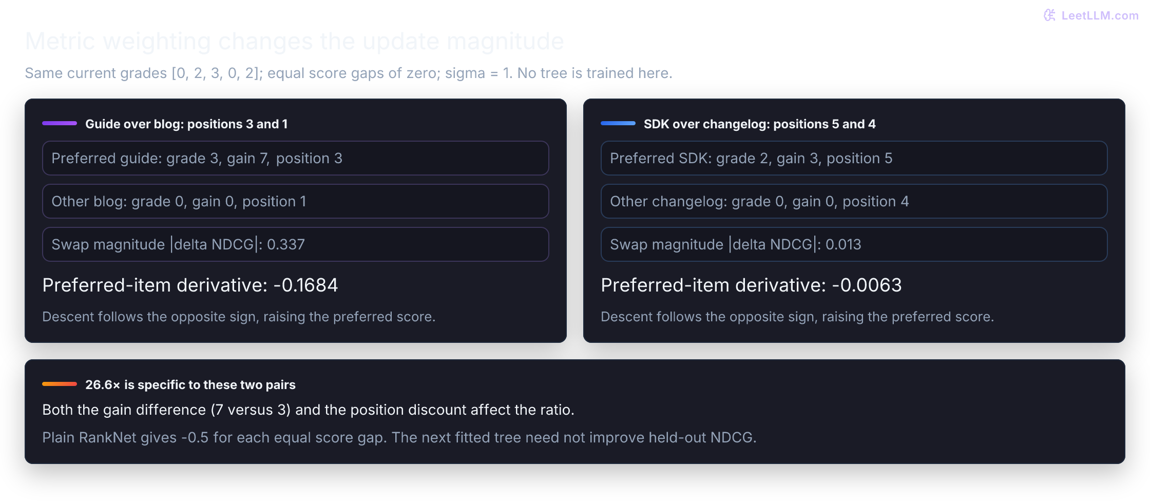
26.6× derivative-magnitude ratio. It doesn't isolate position alone or execute a LambdaMART training run.Each document receives a net weighted score derivative .
Under our derivative convention, descent raises the preferred item's score by following ; the other item receives the opposite direction. Some descriptions call the corrective direction itself a lambda, so record the sign convention.
LambdaMART combines metric-weighted updates with boosted regression trees, including curvature-based leaf updates. Tree fitting aggregates signals across pairs and queries; it doesn't simply weight every split by one swap's delta or differentiate NDCG exactly.[9]
Build pair preferences for our running query.
pairs = [
    (preferred["id"], other["id"])
    for preferred in ranked
    for other in ranked
    if preferred["relevance"] > other["relevance"]
]

print("pair count:", len(pairs))
print("first pairs:", pairs[:5])pair count: 8
first pairs: [('api-guide', 'retry-runbook'), ('api-guide', 'sdk-example'), ('api-guide', 'blog-post'), ('api-guide', 'legacy-changelog'), ('retry-runbook', 'blog-post')]The pair ("api-guide", "blog-post") says the API guide should score higher for this query. Equal grades don't form a pair, so retry-runbook vs sdk-example is absent.
Take one linear RankNet parameter step, then separately calculate two metric-weighted score derivatives. For the latter arithmetic, assume both pairs have zero score gap and use the displayed order as the tie order. No ranker is trained from those two lambdas.
by_id = {item["id"]: item for item in eligible}
preferred, other = by_id["api-guide"], by_id["blog-post"]
feature_names = ("query_fit", "reliability")
difference = [preferred[name] - other[name] for name in feature_names]

def preference_probability(gap):
    if gap >= 0:
        return 1 / (1 + exp(-gap))
    z = exp(gap)
    return z / (1 + z)

def pair_loss(gap):
    return max(0.0, -gap) + log1p(exp(-abs(gap)))

weights = [0.0, 0.0]
gap_before = sum(w * x for w, x in zip(weights, difference))
gradient = [(preference_probability(gap_before) - 1) * x for x in difference]
weights = [w - 0.5 * grad for w, grad in zip(weights, gradient)]
gap_after = sum(w * x for w, x in zip(weights, difference))

def delta_ndcg(grades, pos_i, pos_j, limit=5):
    swapped = list(grades)
    swapped[pos_i], swapped[pos_j] = swapped[pos_j], swapped[pos_i]
    best = dcg(sorted(grades, reverse=True)[:limit])
    return abs(dcg(swapped[:limit]) - dcg(grades[:limit])) / best if best else 0.0

# State: [blog-post(0), retry-runbook(2), api-guide(3), legacy-changelog(0), sdk-example(2)]
misordered_grades = [0, 2, 3, 0, 2]
d_top = delta_ndcg(misordered_grades, 0, 2, 5)
d_bottom = delta_ndcg(misordered_grades, 3, 4, 5)

lambda_top = -0.5 * d_top
lambda_bottom = -0.5 * d_bottom

print("RankNet weight gradient:", [round(g, 4) for g in gradient])
print("RankNet updated weights:", [round(w, 4) for w in weights])
print(f"top swap delta_ndcg: {d_top:.3f} -> preferred derivative: {lambda_top:.4f}")
print(f"bottom swap delta_ndcg: {d_bottom:.3f} -> preferred derivative: {lambda_bottom:.4f}")
print(f"weighted derivative magnitude ratio: {lambda_top / lambda_bottom:.1f}x")RankNet weight gradient: [-0.315, 0.045]
RankNet updated weights: [0.1575, -0.0225]
top swap delta_ndcg: 0.337 -> preferred derivative: -0.1684
bottom swap delta_ndcg: 0.013 -> preferred derivative: -0.0063
weighted derivative magnitude ratio: 26.6xThe one-pair parameter update gives the guide a positive score gap. Separately, the metric-weighted score derivatives differ by 26.6× in magnitude. The guide/blog grade gap is 3 while the SDK/changelog gap is 2, so that ratio reflects gain differences as well as position discounts. Neither pair calculation guarantees that the next fitted tree improves held-out NDCG.
Log exposure before reading clicks
The ranked slate is now ready to display. A click tells you what a developer selected, but not what was never shown.
Record displayed impressions, including unclicked documents, separately from later outcomes. A server's proposed slate isn't proof that a browser rendered it; define the exposure event and collect the corresponding client signal.
The synthetic rows below record a proposed slate and name a snapshot that a production system would have to retain. The code doesn't observe browser rendering or create that snapshot. A real replay record needs candidate IDs, feature values, document versions, and permitted request context. Keep the resulting log protected and subject to retention.
slate = ranked[:3]
impressions = [
    {
        "request_id": "req-1042",
        "shown_at": "2026-05-01T12:00:00Z",
        "replay_snapshot": "docs-request-snapshot-1042",
        "query": query,
        "eligibility_policy": "docs-access-policy-v4",
        "candidate_set": "retrieval-v3",
        "ranker": "docs-ranker-v7",
        "document_id": item["id"],
        "position": position,
    }
    for position, item in enumerate(slate, start=1)
]
outcomes = [
    {
        "event_id": "evt-click-1042",
        "occurred_at": "2026-05-01T12:00:03Z",
        "request_id": "req-1042",
        "document_id": "api-guide",
        "event": "click",
    },
    {
        "event_id": "evt-resolved-1042",
        "occurred_at": "2026-05-01T12:04:18Z",
        "request_id": "req-1042",
        "document_id": "api-guide",
        "event": "resolved",
    },
]

print("slate:", [item["id"] for item in slate])
print("logged positions:", [(row["document_id"], row["position"]) for row in impressions])
print("later outcomes:", [(row["document_id"], row["event"]) for row in outcomes])slate: ['api-guide', 'retry-runbook', 'sdk-example']
logged positions: [('api-guide', 1), ('retry-runbook', 2), ('sdk-example', 3)]
later outcomes: [('api-guide', 'click'), ('api-guide', 'resolved')]The fixture assigns the guide position 1 and supplies later click/resolution events. It doesn't prove a real developer saw it or resolved a task. In a live log, exposure and outcomes remain separate observations.
Log enough context to interpret later outcomes:
| Logged field | Reason |
|---|---|
| request and query ID | group displayed slate and join later outcomes |
| eligibility-policy version | know which documents were allowed |
| candidate IDs and feature snapshot | know what could have ranked and reproduce scores |
| rendered positions and exposure timestamp | record display context; examination remains latent |
| ranker version | attribute outcomes |
| timestamped click, save, resolved events | distinguish curiosity from value |
| freshness and permission snapshot | reproduce context without overriding current access checks |
Protect logs and snapshots carefully: query text can contain secrets, and a hash of a low-entropy query isn't anonymization. Keep only context needed for analysis and enforce retention policies.
Debias click logs with inverse propensity scoring
Position can affect clicks through examination, presentation, and trust. Training on raw clicks can reinforce prior exposure: shown items get more opportunities to accumulate clicks. This can create a feedback loop, not an inevitable permanent lock at the top.[11]
An explicit position-based model
For this simplified model, assume a click requires examination and relevance, with no accidental clicks or other noise. Also assume examination depends only on position, independently of relevance given the request context. These are modeling assumptions, not observed facts:
Let be the examination propensity at rank position .
Raw click-through rate (CTR) conflates examination with relevance. To extract an unbiased estimate of intrinsic relevance , use Inverse Propensity Scoring (IPS):
where is an observed click, and is the correctly specified absolute examination probability for this population. This is an importance-weighted contribution, not a per-impression probability: a click at contributes 10.
Under the stated model, its expectation is the relevance probability:
historical = [
    {"document": "same-quality-a", "position": 1, "impressions": 100, "clicks": 40},
    {"document": "same-quality-b", "position": 2, "impressions": 100, "clicks": 20},
]

for row in historical:
    raw_ctr = row["clicks"] / row["impressions"]
    print(
        f"{row['document']}: position={row['position']} "
        f"raw_ctr={raw_ctr:.2f}"
)same-quality-a: position=1 raw_ctr=0.40
same-quality-b: position=2 raw_ctr=0.20The counts alone show different CTRs; they don't establish equal quality. Now assume absolute propensities 1.0 and 0.5. Applying the correction yields equal sample estimates:
examination_propensity = {1: 1.0, 2: 0.5, 3: 0.1, 4: 0.02}

for row in historical:
    corrected_signal = (
        row["clicks"]
        / examination_propensity[row["position"]]
        / row["impressions"]
    )
    print(f"{row['document']}: corrected_signal={corrected_signal:.2f}")

# Demonstrate propensity truncation for deep positions
deep_row = {"document": "rare-doc-d", "position": 4, "impressions": 100, "clicks": 1}
raw_weight = 1.0 / examination_propensity[deep_row["position"]]
clipped_weight = min(raw_weight, 10.0)
print(f"slot 4 raw inverse weight: {raw_weight:.1f}")
print(f"slot 4 clipped inverse weight: {clipped_weight:.1f}")same-quality-a: corrected_signal=0.40
same-quality-b: corrected_signal=0.40
slot 4 raw inverse weight: 50.0
slot 4 clipped inverse weight: 10.0Real-world propensity estimation and clipping
Randomized position interventions can estimate relative propensities under a suitable click model. Compare the same source population with and without a random swap; its CTR ratio estimates when examination is the relevant position effect and the model remains stable. The original paper uses a landmark position and estimates propensities up to a multiplicative constant, which is enough for its ranking-risk comparisons. It doesn't identify absolute relevance probabilities without an anchor.[11]
If slot 1 is examined with probability 0.8 rather than 1, the same relative ratio implies slot 2 probability 0.4. Predict how both corrected estimates change:
for first_slot_probability in [1.0, 0.8]:
    absolute_probabilities = [first_slot_probability, 0.5 * first_slot_probability]
    estimates = [
        ctr / probability
        for ctr, probability in zip([0.4, 0.2], absolute_probabilities)
    ]
print(f"slot-1 anchor={first_slot_probability:.1f}: estimates={estimates}")slot-1 anchor=1.0: estimates=[0.4, 0.4]
slot-1 anchor=0.8: estimates=[0.5, 0.5]Equal corrected signals don't prove equal intrinsic quality, particularly with finite samples or a misspecified model. Examination correction also doesn't repair missing catalog exposure: an item never retrieved has no observations. A counterfactual policy estimate needs logging-policy coverage of the target actions and their selection probabilities. Those aren't the same as . Randomization must stay within current authorization and product constraints.
Clipping trades bias for variance; the bias needn't be tiny. With p=0.02 and an inverse-weight cap of 10, the expected clipped contribution under this model is , not . A relevance rate 0.5 would therefore yield expected clipped signal 0.1. This limit can stabilize estimation while substantially changing its target. Validate the cap and population assumptions rather than treating it as a free correction.[11]
Why can't raw click rate serve as an unbiased relevance label?
Answer
Users can click only items they were shown, and higher-ranked items receive more attention. Log exposure and position, then use controlled exploration or bias-aware estimation before treating clicks as preference evidence.
Protect users and enforce slate policies
Ranking can narrow what developers see. In this portal, stale documents and private drafts are ineligible. Freshness isn't universally a hard filter: an archive search might deliberately return old documents. State the product rule before encoding it as policy.
A final-slate diversity constraint can be enforced after scoring: if policy permits at most two results from one source in the top three, adjust the slate and gate that invariant. Earlier retrieval may also need multiple sources so the final stage has alternatives to choose from. Define an underfilled-slate fallback if too few eligible sources exist. Monitor new documents, small doc sets, and languages rather than accepting one portal-wide NDCG.
Give the guide, runbook, and SDK example the same source. The other two documents come from a second source. Walk the already scored, eligible list in order, accepting an item only while its source has capacity. Predict which document takes the third slot and what happens to system NDCG.
source_by_id = {
    "api-guide": "platform",
    "retry-runbook": "platform",
    "sdk-example": "platform",
    "blog-post": "community",
    "legacy-changelog": "community",
}

def source_limited_slate(ordered_items, slots, per_source):
    selected = []
    counts = {}
    for item in ordered_items:
        if len(selected) == slots:
            break
        source = source_by_id[item["id"]]
        if counts.get(source, 0) < per_source:
            selected.append(item)
            counts[source] = counts.get(source, 0) + 1
    return selected

constrained = source_limited_slate(ranked, slots=3, per_source=2)
one_source = [item for item in ranked if source_by_id[item["id"]] == "platform"]
underfilled = source_limited_slate(one_source, slots=3, per_source=2)
print("constrained slate:", [item["id"] for item in constrained])
print("system ndcg@3:", f"{system_ndcg(constrained, eligible, 3):.3f}")
print("one-source slate:", [item["id"] for item in underfilled])constrained slate: ['api-guide', 'retry-runbook', 'blog-post']
system ndcg@3: 0.856
one-source slate: ['api-guide', 'retry-runbook']This policy replaces a grade-2 SDK answer with a grade-0 blog, lowering the relevance metric from 1.000 to 0.856. That trade-off needs a product reason; diversity isn't automatically an improvement. With only one source, this example's fallback displays two items. It doesn't fill the missing slot by violating the cap or pulling an ineligible document. The helper assumes unique IDs, known sources, and positive integer limits. It enforces this one source-count rule, not an optimal solution to arbitrary overlapping slate constraints.
Hard authorization must remain enforceable independently of the learned score. Reproduce an unsafe proposed slate by sorting the raw corpus and omitting the eligibility filter.
unsafe_order = sorted(
    corpus,
    key=lambda item: (-rank_score(item), item["id"]),
)

print("unsafe first result:", unsafe_order[0]["id"])
print("permitted:", unsafe_order[0]["permitted"])unsafe first result: private-draft
permitted: FalseThe private draft ranks first because its query match is strong. Computing that score internally isn't itself a disclosure; displaying the unfiltered result would be. Better model training can't establish an access-control guarantee.
Restore the prefilter used by this lab, and test that the final displayed slate obeys current permissions. An authorization change between indexing and serving must not be bypassed by a stale candidate cache.
Gate offline candidates and design online tests
A release review needs both ranking evidence and interpretable outcome logs. Check candidate recall and system NDCG, then use reranker NDCG to isolate ordering errors. Add measured p95 latency, final-slate constraints, and an experiment plan.
A list that looks good offline isn't allowed to silently write its own future training labels.
The following authored fixture checks exercise metric and logging logic. They don't grant release approval:
- candidate recall at
5must be1.0 - reranker NDCG@5 and system NDCG@3 must each be at least
0.95 - the supplied synthetic scorer-time samples have nearest-rank p95 at most
20milliseconds - blocked documents must stay absent
- impression rows must include fields needed for replay
- outcome events must join a logged impression and have unique event IDs
# Authored samples for percentile/gate arithmetic, not timings of this scorer.
latencies_ms = [11, 13, 12, 15, 14, 16, 13, 12, 17, 18]

def percentile_nearest_rank(values, percentile):
    if not values or not 0 < percentile <= 1:
        raise ValueError("provide samples and a percentile in (0, 1]")
    rank = ceil(len(values) * percentile)
    return sorted(values)[rank - 1]

required_impression_fields = {
    "request_id",
    "shown_at",
    "replay_snapshot",
    "query",
    "eligibility_policy",
    "candidate_set",
    "ranker",
    "document_id",
    "position",
}
required_outcome_fields = {
    "event_id",
    "occurred_at",
    "request_id",
    "document_id",
    "event",
}
exposed_keys = {
    (row["request_id"], row["document_id"])
    for row in impressions
}
release_checks = {
    "candidate_recall_at_5": candidate_recall(candidates) >= 1.0,
    "reranker_ndcg_at_5": reranker_ndcg(ranked, 5) >= 0.95,
    "system_ndcg_at_3": system_ndcg(ranked, eligible, 3) >= 0.95,
    "p95_latency_ms": percentile_nearest_rank(latencies_ms, 0.95) <= 20,
    "blocked_items_absent": not (
        {"private-draft", "stale-guide"}
        & {item["id"] for item in ranked}
    ),
    "impression_schema": bool(impressions) and all(
        required_impression_fields <= row.keys()
        for row in impressions
    ),
    "outcome_schema": all(
        required_outcome_fields <= row.keys()
        for row in outcomes
    ),
    "outcomes_join_impressions": all(
        (row["request_id"], row["document_id"]) in exposed_keys
        for row in outcomes
    ),
    "unique_outcome_events": len({row["event_id"] for row in outcomes}) == len(outcomes),
}

for name, passed in release_checks.items():
    print(f"{name}: {passed}")
print("fixture checks:", all(release_checks.values()))
assert all(release_checks.values())candidate_recall_at_5: True
reranker_ndcg_at_5: True
system_ndcg_at_3: True
p95_latency_ms: True
blocked_items_absent: True
impression_schema: True
outcome_schema: True
outcomes_join_impressions: True
unique_outcome_events: True
fixture checks: TrueThe checks pass on one hand-assigned query and ten authored latency values. The nearest-rank sample p95 is their maximum, 18; it isn't a measured population p95. Required-field presence doesn't validate field types, clock order, rendering, snapshot retention, or policy freshness. These gates evaluate the original unconstrained order; promoting the separate source-constrained slate would also require a source-cap gate and metrics for that final slate. None of these fixture results establishes readiness for an online experiment.
A real candidate needs representative held-out queries and slices, measured serving performance, current authorization checks, actual replay evidence, and an experiment review. Engagement changes can reflect latency, layout, freshness, source trust, and ranking behavior.
Use randomized A/B assignment, as in Experiment Design and A/B Testing, rather than comparing two time windows.[12] Here assignment is by developer, so repeated sessions from the same developer aren't independent experimental units. Analyze at the developer level or use uncertainty estimates that account for clustering.
Predeclare enrollment, metric, sample size, duration, uncertainty method, and decision rule. The illustrative numbers below aren't a power calculation. Assign developers at their first eligible request and keep assignment stable. Define the analysis window and resolution-event attribution, including timeout and missing-event handling. A mean of developer-level session ratios weights developers equally; it isn't the pooled resolved-session rate.
Meeting a minimum isn't permission to repeatedly test until significance appears. The proposed plan makes one efficacy analysis after both exposure requirements are met; safety monitoring can stop harmful exposure earlier. It still lacks an effect size, significance/power targets, and a complete success rule.
Record the proposed plan before real exposure. This fixture receipt documents calculations and illustrative experiment fields, not a published model or complete experiment protocol.
receipt = {
    "artifact": "docs-ranker-v7",
    "evidence_type": "synthetic_fixture",
    "operational_status": "not_evaluated",
    "eligibility_policy": "docs-access-policy-v4",
    "candidate_set": "retrieval-v3",
    "offline": {
        "candidate_recall_at_5": round(candidate_recall(candidates), 3),
        "reranker_ndcg_at_5": round(reranker_ndcg(ranked, 5), 3),
        "system_ndcg_at_3": round(system_ndcg(ranked, eligible, 3), 3),
        "p95_latency_ms": percentile_nearest_rank(latencies_ms, 0.95),
    },
    "release_checks": release_checks,
    "required_checks_pass": all(release_checks.values()),
    "experiment": {
        "assignment_unit": "developer_id",
        "analysis_unit": "developer_id",
        "control": "docs-ranker-v6",
        "treatment": "docs-ranker-v7",
        "primary_metric": "mean_developer_resolution_rate",
        "metric_definition": "resolved sessions / all sessions for each developer, then mean over developers",
        "minimum_duration_days": 14,
        "minimum_developers_per_arm": 5000,
        "analysis_schedule": "one efficacy analysis after both minimums; no significance peeking",
        "guardrails": [
            "bad_result_reports_per_session",
            "p95_latency_ms",
            "blocked_document_impressions",
        ],
        "safety_stops": {
            "blocked_document_impressions": 0,
            "p95_latency_ms": 20,
        },
    },
    "status": "fixture_checks_passed" if all(release_checks.values()) else "fixture_checks_failed",
}
payload = dumps(receipt, sort_keys=True)
print("status:", receipt["status"])
print("offline:", receipt["offline"])
print("receipt sha256:", sha256(payload.encode()).hexdigest()[:12])status: fixture_checks_passed
offline: {'candidate_recall_at_5': 1.0, 'reranker_ndcg_at_5': 1.0, 'system_ndcg_at_3': 1.0, 'p95_latency_ms': 18}
receipt sha256: b569fb7aabb2The receipt's short hash fingerprints this JSON, not scorer bytes, a retained snapshot, or real traffic. Bind actual data/judgment IDs, scorer revision, dependencies, index/tower versions, and validation evidence before promoting a real candidate. The offline p95 field describes supplied scorer samples; the proposed live p95 guardrail needs a clearly defined measurement scope and window.
Common ranking failure modes and debugging
Use the first broken boundary to choose your next measurement. A strong reranker score can't compensate for a missing candidate, a policy bypass, or an outcome log that can't join back to exposure.
| Symptom | Probable cause | Fix |
|---|---|---|
| NDCG looks strong but desired document never appears | Candidate retrieval lost recall | Measure retrieval recall and system NDCG separately from reranker NDCG |
| Prohibited document is displayed | Authorization was absent, stale, or bypassed | Enforce current eligibility pre-filters and gate blocked impressions |
| Popular documents dominate the slate | Exposure/position feedback, candidate coverage, or genuinely strong demand | Inspect retrieval coverage and click-model assumptions; evaluate constrained exploration and propensity weighting |
| Corrected click score still looks suspicious | Propensity estimate is wrong | Validate click model or collect randomized intervention data |
| Corrected click score becomes unstable | Tiny propensities create large inverse weights | Check support and model fit; evaluate clipping's bias/variance trade-off |
| CTR improves while bad-result reports rise | Clickbait objective mismatch | Pair engagement with task resolution and explicit negative feedback guardrails |
Each row is a hypothesis to investigate, not a diagnosis established by the symptom alone. A falling click rate could reflect worse ranking, a changed interface, or quick task completion.
Try changing one assumption
Work in a copy of the lab so each change starts from the original fixture.
- Set the candidate budget to
4, rerank those candidates, and evaluate at cutoff3. Predict candidate recall, reranker NDCG, and system NDCG before calculating them. - Swap
api-guideandretry-runbookin the original ranked list. Which changes: candidate recall, NDCG@3, or both? - In the one-pair update, reverse the preference while keeping zero initial weights. What happens to the two weight-gradient signs? Check that the newly preferred document gains a positive score gap.
- Add an outcome for a document absent from
impressions. Separately, duplicate an existing outcome'sevent_id. Which gate should fail for each change?
Check your predictions
- Four candidates include the guide and runbook but miss the SDK example: recall is
2/3. Their best order has grades[3, 2, 0], giving reranker NDCG@31.000but system NDCG@3 about0.856. The whole-corpus ideal remains[3, 2, 2]. - Recall stays
1.000because no document leaves the candidate set. The reordered grades[2, 3, 2]give NDCG@3 about0.858: the grade-3 answer loses more from moving down than the grade-2 answer gains from moving up. - The feature difference becomes
[-0.63, 0.09]; the gradient becomes[0.315, -0.045]and the updated weights[-0.1575, 0.0225]. The update follows the supplied label, even when that label contradicts the judgment you intended. - The orphan event fails
outcomes_join_impressions. A repeated event ID failsunique_outcome_events, even though both copies join an impression. Joinability and deduplication protect different failure modes.