Personalize this lesson
Adapt explanations and teaching visuals to your background and preferred voice.
An operator asks, How do I rotate an API key? A search service has already embedded that question and its documentation. One scoring rule puts the rotation guide first; another favors a longer vector. Compress the vectors to save memory, and the ranking can change again. What exactly changed: the definition of similarity, or its approximation?
Sentence embeddings explained how training shapes an embedding space. Here the encoder stays fixed while we examine the numbers used to search it. All small vectors below are hand-constructed examples, not outputs from a trained model. The document names keep the retrieval task recognizable; their coordinates change between experiments to isolate different effects.
Our target passage is api-key-rotation-v3. A private incident note also appears in diagnostic comparisons, but similarity is never an access-control check: unauthorized rows must be excluded from evidence regardless of their score. First establish the geometry, then measure what shorter vectors and lower-precision quantization preserve.
Three ways to measure closeness
Start with one small question: what should "close" mean for these two chunks? An embedding is a point in high-dimensional space, represented by a list of numbers from the encoder. Three common rulers answer different versions of that question.
| Ruler | Question | Range | Scaling one document by a positive factor |
|---|---|---|---|
| Cosine similarity | Do they point the same way? | to | No |
| Dot product | How much do matching coordinates reinforce each other? | to | Can change rank |
| Euclidean (L2) distance | What's the straight-line gap? | to | Can change rank |
Positive scaling preserves a nonzero vector's direction. Negative scaling reverses it, and scaling to zero makes cosine undefined. If every stored vector and query has length 1, descending cosine, descending dot product, and ascending L2 distance give the same exact ranking. Approximate indexes can still return different candidates.
A zero vector is the exception you have to reject explicitly: cosine divides by both vector norms, so a zero-norm query has no defined direction. Replacing that division with an arbitrary zero score can quietly reorder an entire shortlist. Record the encoder failure and refuse retrieval instead of pretending the query matched nothing.
A tiny 2D example makes the split visible. Two paraphrases of the rotation guide map to:
- Passage A,
api-key-rotation-v3:[3, 4] - Passage B, a second rotation phrasing:
[4, 3]
These coordinates put the vectors in nearby directions, but neither “northeast” nor a raw dot score establishes relevance. Work out the three scores before deciding how to rank a larger candidate set.
Keep this equal-length pair in mind. Later fixtures will make the less obvious case visible: same direction, different length.
Cosine similarity
Multiply matching dimensions and add:
The length of a vector is the square root of the sum of squared components:
Their lengths are both 5, so now divide by :
That length-corrected dot product is cosine similarity. For any two nonzero vectors:
1 means the same direction, 0 means orthogonal, and -1 means opposite. That's a geometry result, not a relevance guarantee. Whether the direction tracks useful matches still depends on the encoder and retrieval evaluation.
Dot product
Now remove the length correction. Dot product stops at the sum we already computed:
Here the dot product is positive, so increasing A's length increases that score. In general, positive scaling multiplies the dot score: a negative score becomes more negative, not larger. If all candidate norms are equal, dividing by their shared norm preserves their ranking; otherwise raw dot product and cosine can disagree.
Euclidean distance
The third ruler asks for the straight-line gap. Subtract, square, sum, and take the square root:
The distance is about 1.41 in this coordinate system. Calling that “small” needs a comparison set; it isn't a universal relevance threshold. With different candidate norms, L2 and cosine can rank that set differently.
You've worked the numbers. Predict the next output: after A is scaled by 10, should cosine change, should dot product change, or should both stay fixed? This snippet checks the hand math and makes that prediction concrete:
import math

passage_a = [3.0, 4.0]
passage_b = [4.0, 3.0]

def dot(left: list[float], right: list[float]) -> float:
    return sum(x * y for x, y in zip(left, right, strict=True))

def l2_norm(vector: list[float]) -> float:
    return math.hypot(*vector)

score = dot(passage_a, passage_b)
cosine = score / (l2_norm(passage_a) * l2_norm(passage_b))
euclidean = l2_norm([x - y for x, y in zip(passage_a, passage_b, strict=True)])
print(f"dot={score:.0f}, cosine={cosine:.2f}, euclidean={euclidean:.2f}")

longer_a = [10.0 * value for value in passage_a]
same_direction_cosine = dot(longer_a, passage_b) / (
    l2_norm(longer_a) * l2_norm(passage_b)
)
print(f"10x vector: cosine={same_direction_cosine:.2f}, dot={dot(longer_a, passage_b):.0f}")dot=24, cosine=0.96, euclidean=1.41
10x vector: cosine=0.96, dot=240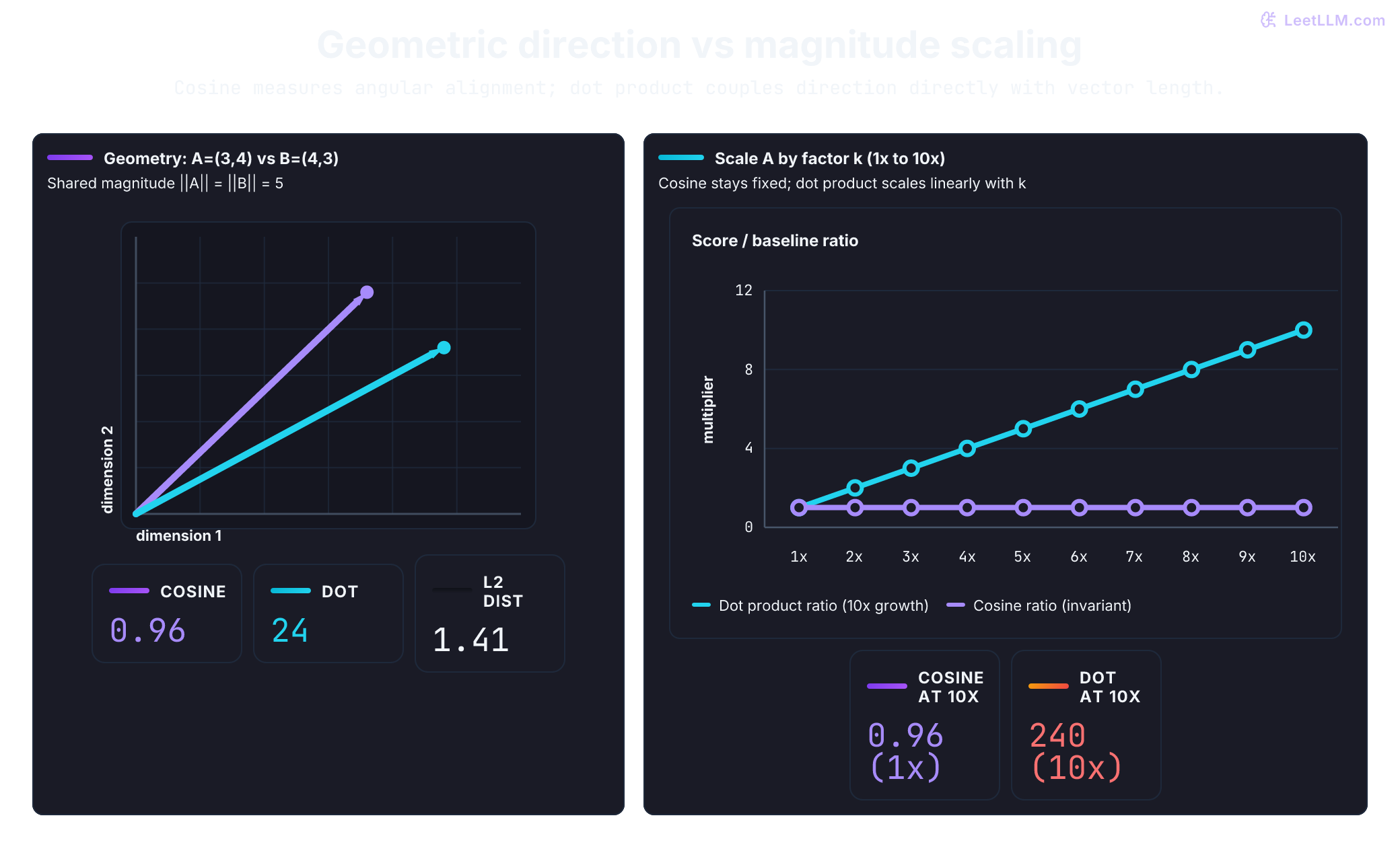
If vector A is [3, 4] and vector C is [30, 40], what happens to cosine similarity and dot product when you compare both vectors to [4, 3]?
Answer
Cosine similarity stays the same because A and C point in the same direction. Dot product grows by 10x because C is 10x longer. Cosine ignores magnitude. Dot product keeps it.
The experiment gives you a serving decision. Use cosine when the model card, training setup, or labeled queries say length shouldn't change rank. Use raw dot product when magnitude is part of the learned score, as in maximum inner product search (MIPS).
If every vector is already unit length, the rankings match and inner product avoids norm divisions while scoring candidates.
When the three rulers agree
The first fixture used equal-length vectors. Real encoders don't promise that unless their documentation or your pipeline says so. Treat normalization as an explicit contract shared by model output, index construction, and query serving. Don't infer it from a model name.
With that contract in place, the three rulers collapse to one ranking. When both vectors have length 1, the cosine denominator is , so cosine equals raw dot product. Squared Euclidean distance becomes a strictly decreasing linear function of that same inner product:
Because both vectors are unit-normalized ( and ), those squared norms simplify directly:
Rearranging gives the exact geometric connection:
For example, unit-vector dot scores of 0.73 and 0.60 correspond to squared Euclidean gaps of and . The larger dot score has the smaller distance. Minimizing straight-line gap on the unit hypersphere is mathematically identical to maximizing cosine similarity or inner product.
Higher inner product, higher cosine, and smaller squared L2 distance now induce the same ranking. Normalize stored rows once and each incoming query once. Candidate scoring can use a fast matrix-multiply kernel without repeated norm divisions.[1]
Here's the failure in the opening story. The next fixture gives private-incident-note-44 a huge raw norm, so it wins unnormalized dot product even though its direction is less aligned with the query. Before running it, predict which label each score will choose. Then compare raw dot, normalized dot, and cosine.
import math

labels = ["api-key-rotation-v3", "private-incident-note-44", "service-token-lifecycle-v2"]
documents = [
    [0.95, 0.05],  # Direction closely matches the rotation query.
    [8.00, 6.00],  # Large norm lets raw dot product dominate.
    [0.20, 0.90],
]
query = [1.0, 0.0]

def dot(left: list[float], right: list[float]) -> float:
    return sum(x * y for x, y in zip(left, right, strict=True))

def l2_normalize(vector: list[float]) -> list[float]:
    if not vector or not all(math.isfinite(value) for value in vector):
        raise ValueError("expected a nonempty finite vector")
    scale = max(abs(value) for value in vector)
    if scale == 0:
        raise ValueError("zero vector has no cosine direction")
    # Scale first so squaring very large or tiny finite values is unnecessary.
    scaled = [value / scale for value in vector]
    norm = math.hypot(*scaled)
    return [value / norm for value in scaled]

def l2_norm(vector: list[float]) -> float:
    return math.hypot(*vector)

raw_dot = [dot(row, query) for row in documents]
unit_documents = [l2_normalize(row) for row in documents]
unit_query = l2_normalize(query)
unit_dot = [dot(row, unit_query) for row in unit_documents]
raw_cosine = [
    dot(row, query) / (l2_norm(row) * l2_norm(query))
    for row in documents
]
unit_squared_l2 = [sum((x - y) ** 2 for x, y in zip(row, unit_query, strict=True)) for row in unit_documents]
assert all(math.isclose(distance, 2 - 2 * score, abs_tol=1e-12)
           for distance, score in zip(unit_squared_l2, unit_dot, strict=True))
for invalid in [[], [0.0, 0.0], [float("nan"), 1.0], [float("inf"), 1.0]]:
    try:
        l2_normalize(invalid)
    except ValueError:
        pass
    else:
        raise AssertionError("invalid direction was accepted")
for extreme in [[1e308, 1e308], [1e-308, 1e-308]]:
    assert math.isclose(l2_norm(l2_normalize(extreme)), 1.0)

print(f"raw dot winner: {labels[raw_dot.index(max(raw_dot))]}")
print(f"normalized winner: {labels[unit_dot.index(max(unit_dot))]}")
print(
    "cosine equals unit dot: "
    f"{all(abs(left - right) < 1e-6 for left, right in zip(raw_cosine, unit_dot, strict=True))}"
)raw dot winner: private-incident-note-44
normalized winner: api-key-rotation-v3
cosine equals unit dot: TrueA large-norm vector isn't automatically junk. The narrower conclusion is about serving: if the contract is cosine-like ranking, skipping normalization changes what the index optimizes.
The code rejects empty, zero, and non-finite vectors and checks extreme finite magnitudes. A finite, nonzero query can be left unnormalized if you only need an inner-product ranking against unit document vectors: its norm multiplies every score equally. Normalize it too when you need cosine values, shared thresholds, or the unit-vector L2 identity. None of these choices authorizes the private note.
L2 distance isn't automatically wrong in high dimension either. On unit vectors, squared L2 produces the same ranking through the identity above. Without normalization, L2 also includes norm differences. Keep it when the model, index, and evaluation were built around that geometry.
The original product-quantization formulation approximates this squared L2 distance between a full-precision query and compressed database vectors.[2]
We've fixed what "close" means. The next pressure is capacity: how many coordinates can you afford to keep before the scoring contract becomes too expensive?
Choosing how many dimensions you need
We've chosen a scoring contract. Now ask what that contract costs. Width controls how much of the trained representation you store, along with memory traffic and scoring work.
A dimension count has no universal quality meaning: a 512-dimensional model trained for your API-doc queries can beat a different 1,536-dimensional model. Compare widths only after holding model family, scoring convention, corpus, and evaluation set fixed.
| Choice under evaluation | What you can conclude | What you still must measure |
|---|---|---|
| Full trained width | Baseline payload and retrieval score for this model | Latency, RAM, and evidence recall |
| Model-supported shorter prefix | Lower raw payload for the same family | Recall loss and failure slices |
| Different smaller model | Possibly cheaper candidate system | Everything again; training changed too |
The table separates two decisions that are easy to conflate. Dimension count changes capacity. Normalization changes score meaning. A supported shorter vector still needs the serving normalization contract documented by its model or applied by your pipeline.
For one representation family, extra dimensions buy capacity but charge the same predictable systems costs:
- Storage. Each float32 is 4 bytes. 1M vectors at 1536d is about 5.7 GiB of raw payload.
- Exact scoring work. A dot product or L2 comparison does linear work in the number of dimensions, written , per candidate.
- Memory bandwidth. Loading vectors from memory can bottleneck approximate nearest neighbor (ANN) search, which finds close vectors without scanning every row.
- End-to-end latency. Halving dimensions doesn't promise halved latency. Graph traversal, filters, networking, and reranking still take time, so measure before you pay or save the memory bill.
Matryoshka prefixes still need a recall test
Suppose memory pressure makes you want 256 dimensions instead of 1,536. Should the first 256 coordinates be useful by accident, or should the model have been trained to put signal there?
Matryoshka Representation Learning (MRL) answers the second question: training minimizes a weighted sum of losses at selected truncation widths , so those prefixes are meant to work on their own.[3]
That's different from post-hoc PCA, which projects already-trained vectors into a smaller linear subspace, usually by preserving variance on a fixed dataset. PCA can still help frozen embeddings. MRL fits a serving path with several dimension budgets when the model was trained for truncation.
Hosted APIs can expose a supported shortening control without you slicing tensors by hand. Checked October 10, 2026, OpenAI's embeddings guide documents a dimensions parameter for text-embedding-3 models, with defaults of 1,536 for text-embedding-3-small and 3,072 for text-embedding-3-large.[4]
The same guide reports that a text-embedding-3-large vector shortened to 256 dimensions outperforms unshortened text-embedding-ada-002 at 1,536 dimensions on MTEB. That's a provider benchmark, not a promise that a 256-d prefix will retrieve api-key-rotation-v3 for your queries.
If you cut a prefix from an already generated vector, normalize that sliced prefix before using unit-vector scoring, then apply the same operation to queries. OpenAI recommends its dimensions parameter and also documents manual slicing with renormalization. For other models, verify which widths and shortening operations they support.[4]
This local check enforces the contract without an API call:
full_embedding = [0.21, -0.05, 0.44, 0.31, 0.18, -0.27, 0.12, 0.09]
short_embedding = l2_normalize(full_embedding[:4])
norm = l2_norm(short_embedding)
assert math.isclose(norm, 1.0)
print(f"dims={len(short_embedding)}, norm={norm:.3f}")dims=4, norm=1.000Normalization restores a unit-vector scoring contract, unless the retained prefix is all zeros, which the helper rejects. It can't restore coordinates you threw away. In the next diagnostic fixture, the last two dimensions distinguish the passages. Cut to width 2 and the private note ties the guide. A deterministic first-row tie-break picks the private note. That's a ranking failure to examine, not permission to serve it.
![Full 4-d fixture: rotation query [1,0,0,1] matches api-key-rotation-v3. After keeping only d0 and d1, that query matches private-incident-note-44 because both rows collapse to [1,0].](/cdn/content-image/fundamentals/embeddings-cosine-dot-product-quantization/illustrations/_generated/matryoshka_dimensions_dark.png?v=90d4a22a1743)
labels = ["private-incident-note-44", "api-key-rotation-v3", "service-token-lifecycle-v2"]
documents = [
    [1.0, 0.0, 1.0, 0.0],
    [1.0, 0.0, 0.0, 1.0],
    [0.0, 1.0, 0.0, 1.0],
]
queries = [
    [1.0, 0.0, 0.0, 1.0],
    [0.0, 1.0, 0.0, 1.0],
]
expected = ["api-key-rotation-v3", "service-token-lifecycle-v2"]

def top1_at_width(width: int) -> list[str]:
    if type(width) is not int or not 1 <= width <= len(documents[0]):
        raise ValueError("width must be within the original embedding")
    docs = [l2_normalize(row[:width]) for row in documents]
    asks = [l2_normalize(row[:width]) for row in queries]
    winners: list[str] = []
    for ask in asks:
        scores = [dot(ask, row) for row in docs]
        winners.append(labels[scores.index(max(scores))])
    return winners

full = top1_at_width(4)
short = top1_at_width(2)
full_recall = sum(got == want for got, want in zip(full, expected, strict=True)) / len(expected)
short_recall = sum(got == want for got, want in zip(short, expected, strict=True)) / len(expected)
assert full_recall == 1.0 and short_recall == 0.5
print(f"full top-1 recall={full_recall:.1%}, results={full}")
print(f"short top-1 recall={short_recall:.1%}, results={short}")full top-1 recall=100.0%, results=['api-key-rotation-v3', 'service-token-lifecycle-v2']
short top-1 recall=50.0%, results=['private-incident-note-44', 'service-token-lifecycle-v2']This isn't a benchmark for a real MRL model. Each query has one labeled relevant passage, so the average top-1 hit indicator equals mean Recall@1 here. For multiple relevant passages, Recall@K is the fraction of those passages retrieved in the first K results. Separately measure ANN recall against exact-search neighbors; reproducing a nearest neighbor doesn't prove that neighbor is relevant. Apply the same authorization filter to both sides of a production comparison.
You shorten a unit-normalized 3072-dimensional embedding by taking only the first 256 values. Should you index that prefix immediately?
Answer
No. Verify that the model supports the target width and evaluate held-out retrieval. For a unit-vector scoring contract, normalize nonzero document and query prefixes; reject or explicitly handle zero prefixes. Normalization restores length, not the discarded information.
The memory problem: a sizing example
The prefix test exposed a quality budget. Now put a number on the memory budget. Use the default text-embedding-3-small width of 1,536 dimensions and ask what one million rows cost before graph links, metadata, or replicas.
Scenario: 1 million embeddings, 1,536 dimensions, stored as 32-bit floats (FP32). Predict the raw payload first. Then we'll replace four-byte floats with one-byte values and finally with PQ IDs.
Step 1: the FP32 baseline
Each dimension is a float32, which takes 4 bytes. Multiply rows, dimensions, and bytes per value:
That's only the raw numbers. Real indexes add graph links, metadata, and replicas, but the vector payload alone is already over 5.7 GiB. If that's too large for hot memory, precision is the next lever.
Step 2: 8-bit scalar quantization
Map each float32 to a single byte (INT8). The row count and width stay fixed, so storage drops by about 4x:
Step 3: product quantization
Split each 1,536-dimensional vector into 96 subvectors and store one 8-bit centroid ID per subvector. The compressed row is 96 bytes:
That's a 64x cut in per-row code payload. The PQ codebooks are shared, not free: 96 subspaces × 256 centroids × 16 float32 coordinates require 1,572,864 bytes (1.5 MiB). If you retain FP32 vectors for rescoring, those 5.72 GiB still exist somewhere; compression may save hot RAM without eliminating total storage.
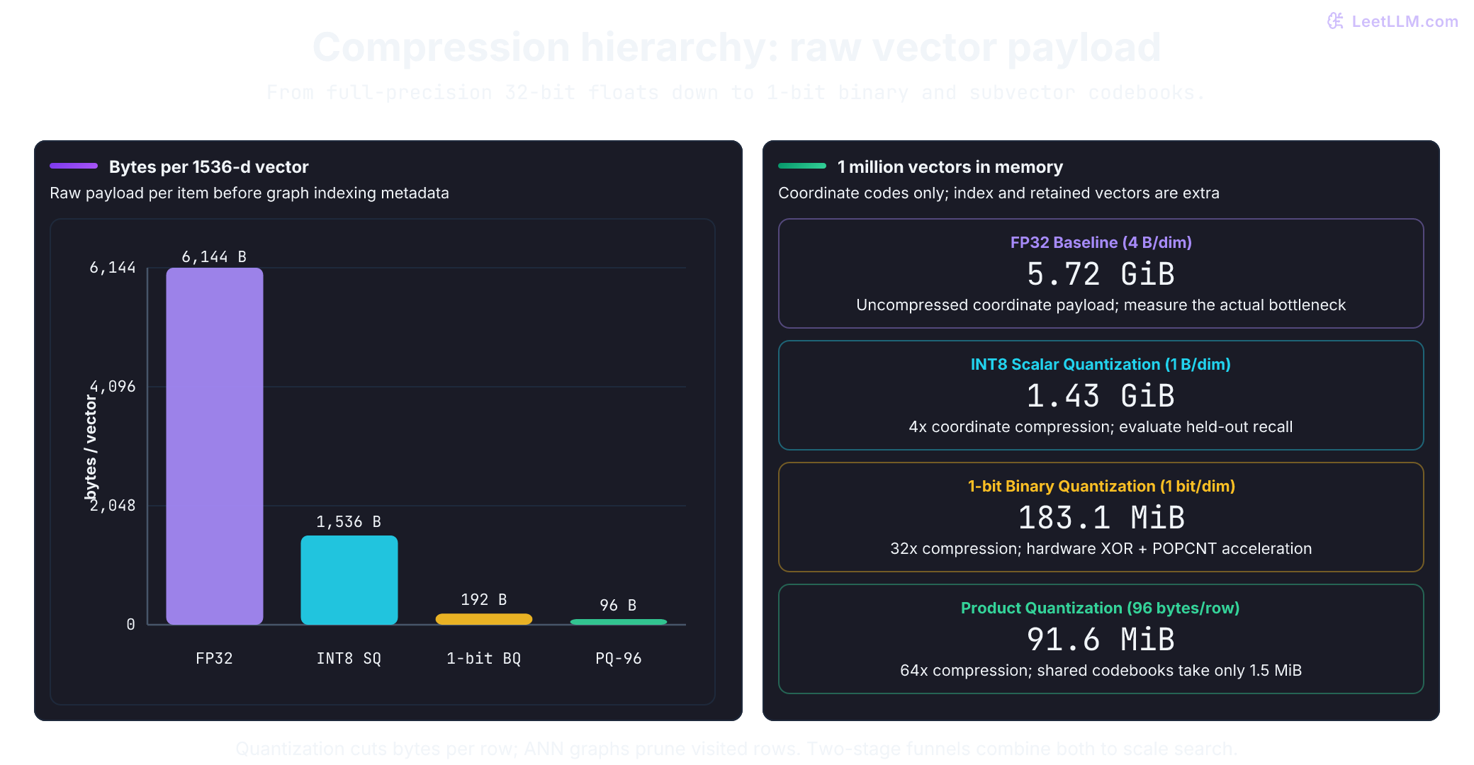
The byte math is easy to turn into a sizing helper. Decimal gigabytes divide by ; binary gibibytes divide by . Label the unit explicitly because storage tools differ:
def payload_bytes(num_vectors: int, bytes_per_vector: int) -> int:
    return num_vectors * bytes_per_vector

raw_bytes = payload_bytes(1_000_000, 1_536 * 4)
int8_bytes = payload_bytes(1_000_000, 1_536)
pq_bytes = payload_bytes(1_000_000, 96)
codebook_bytes = 96 * 256 * (1_536 // 96) * 4
binary_bytes = payload_bytes(1_000_000, (1_536 + 7) // 8)
assert codebook_bytes == 1_572_864
assert raw_bytes // pq_bytes == 64
assert raw_bytes // binary_bytes == 32

print(f"FP32={raw_bytes / 1e9:.2f} GB ({raw_bytes / 1024**3:.2f} GiB)")
print(f"INT8={int8_bytes / 1e9:.2f} GB ({int8_bytes / 1024**3:.2f} GiB)")
print(f"PQ={pq_bytes / 1024**2:.1f} MiB")
print(f"shared_PQ_codebooks={codebook_bytes / 1024**2:.1f} MiB")
print(f"binary_codes={binary_bytes / 1024**2:.1f} MiB")FP32=6.14 GB (5.72 GiB)
INT8=1.54 GB (1.43 GiB)
PQ=91.6 MiB
shared_PQ_codebooks=1.5 MiB
binary_codes=183.1 MiBRe-embedding cost scales with total input tokens, not document count alone. Compute it as total_tokens / 1_000_000 * embedding_price_per_1M_tokens, using the current price for the model you selected.
Keep model version, dimensions, normalization, and quantization settings alongside every index. Otherwise a migration can mix vectors that no longer share a scoring contract.
Shrinking vectors without losing the hit
The sizing math says where the pressure comes from. An exact scan touches up to values. An ANN index reduces how many rows you visit, while quantization reduces bytes per row. Those are separate shortcuts, and either can lose the approved guide, so each needs its own evaluation gate.
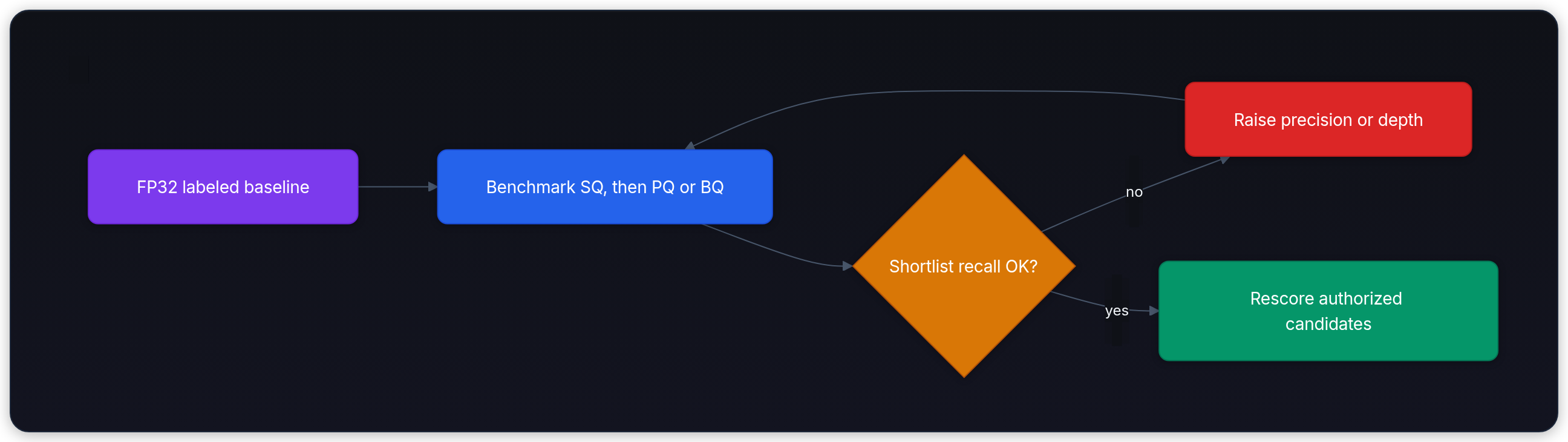
If the FP32 baseline fits RAM and latency, it may be sufficient. Otherwise change one approximation at a time and measure which relevant passages leave the shortlist. Apply authorization before candidate selection when the index supports it; always recheck before fetching text or sending it to a reranker or generator. Post-filtering alone can leave too few usable results.
Scalar quantization (SQ)
Scalar quantization (SQ8) replaces each 32-bit float (4 bytes) with an 8-bit integer (1 byte), giving a 4x reduction in coordinate payload, before scales and index overhead. In this symmetric signed scheme, each dimension is mapped linearly around zero using its calibration scale :
Here over the calibration values for that dimension, with a separate rule for a constant-zero dimension. This scheme uses 255 levels from -127 through 127, leaving -128 unused. With one shared scale for all dimensions, approximate inner-product scoring is:
An alternative is a range-offset quantizer. For a nonconstant interval , map its endpoints to the unsigned codes 0 and 255:
The offset is a real value, not necessarily a representable integer zero-point. An integer-zero-point codec instead specifies a rule such as and , with inside the code domain. Its calibration must account for that restriction. Mixing the two formulas changes the reconstruction. For per-dimension range offsets, a dot score is . Shared offsets add the same query-specific constant to every row, so you may omit that constant for a fixed-query ranking when all rows share calibration. Keep it for score values and thresholds; document-specific offsets do not cancel this way.
Signed storage does not imply symmetric calibration. Sentence Transformers documents per-dimension min/max buckets and both signed and unsigned byte formats.[5] Qdrant describes its scalar codec as float32 -> uint8.[6] Follow the selected codec's range, rounding, clipping, offset, and scoring rules instead of assuming every engine uses the symmetric helper below.
For example, an interval has . Its range-offset codec can represent both endpoints. The quantity is not a valid unsigned-byte zero-point. If exact zero representation is required, expand the calibration interval to include zero, which sacrifices some resolution over .
a, b = 2.0, 3.0
step = (b - a) / 255
endpoint_codes = [round((value - a) / step) for value in (a, b)]
reconstructed = [a + step * code for code in endpoint_codes]
invalid_zero_point = round(-a / step)
zero_inclusive_step = (b - 0.0) / 255
assert endpoint_codes == [0, 255] and reconstructed == [2.0, 3.0]
assert not 0 <= invalid_zero_point <= 255
print("endpoint codes:", endpoint_codes, "reconstructed:", reconstructed)
print("proposed byte zero-point:", invalid_zero_point, "(outside 0..255)")
print(f"step over [2,3]={step:.6f}; step over [0,3]={zero_inclusive_step:.6f}")endpoint codes: [0, 255] reconstructed: [2.0, 3.0]
proposed byte zero-point: -510 (outside 0..255)
step over [2,3]=0.003922; step over [0,3]=0.011765Fit ranges on representative calibration vectors, freeze them, and use the same ranges to encode later rows. Sentence Transformers accepts explicit ranges or calibration embeddings instead of deriving ranges from a small query batch.[5]
The next cell separates fitting scales from encoding. It also packs codes into an actual signed-byte array: a Python list of integers isn't an INT8 storage format. The three-row sample makes the mechanics visible, not a sufficient production calibration set.
from array import array
import math

vectors = [
    [0.20, -1.00, 2.50],
    [0.24, -0.80, 2.10],
    [0.50, -1.40, 2.30],
]

def validate_rows(rows: list[list[float]]) -> int:
    if not rows or not rows[0]:
        raise ValueError("expected a nonempty matrix")
    width = len(rows[0])
    if any(len(row) != width for row in rows):
        raise ValueError("ragged vectors")
    if any(not math.isfinite(value) for row in rows for value in row):
        raise ValueError("non-finite coordinate")
    return width

def fit_scales(rows: list[list[float]]) -> list[float]:
    width = validate_rows(rows)
    max_abs = [max(abs(row[dim]) for row in rows) for dim in range(width)]
    # A constant-zero dimension encodes as zero; scale 1 avoids division by zero.
    return [bound / 127 if bound else 1.0 for bound in max_abs]

def encode_int8(rows: list[list[float]], scales: list[float]) -> list[list[int]]:
    width = validate_rows(rows)
    if len(scales) != width or any(not math.isfinite(s) or s <= 0 for s in scales):
        raise ValueError("expected one positive finite scale per dimension")
    return [
        [
            round(max(-127.0, min(127.0, row[dim] / scales[dim])))
            for dim in range(width)
        ]
        for row in rows
    ]

scale = fit_scales(vectors)
codes = encode_int8(vectors, scale)
reconstructed = [
    [scale[dim] * code for dim, code in enumerate(row)]
    for row in codes
]
max_error = max(
    abs(original - approx)
    for original_row, approx_row in zip(vectors, reconstructed, strict=True)
    for original, approx in zip(original_row, approx_row, strict=True)
)
packed = array("b", [code for row in codes for code in row])
assert packed.itemsize == 1 and len(packed.tobytes()) == 9
assert encode_int8([[0.0, 0.0]], fit_scales([[0.0, 0.0]])) == [[0, 0]]
assert encode_int8([[100.0, -100.0, 0.0]], scale)[0][:2] == [127, -127]
for invalid in [[], [[]], [[1.0], [1.0, 2.0]], [[float("nan")]]]:
    try:
        fit_scales(invalid)
    except ValueError:
        pass
    else:
        raise AssertionError("invalid calibration matrix accepted")
print(f"codes[0]={codes[0]}, max_error={max_error:.4f}")
print(f"packed_code_bytes={len(packed.tobytes())}; scales_stored_separately={len(scale)}")codes[0]=[51, -91, 127], max_error=0.0063
packed_code_bytes=9; scales_stored_separately=3Python's round uses ties-to-even; a production codec may define another rounding rule. The nine packed coordinates occupy nine bytes, but scales, array headers, document IDs, and index structures add storage. The helper rejects unusable scales instead of silently accepting underflow to zero. A coordinate that was always zero during calibration may later become nonzero, so monitor drift and clipping.
INT8 doesn't promise any fixed Recall@K. Model distribution, calibration sample, scoring rule, shortlist depth, and reranking all change the observed loss.
Per-dimension scales also belong in the score. With a full-precision query, approximate dot product is the sum of query[j] * scale[j] * code[j]. Dropping scale[j] changes the relative importance of coordinates. If both operands are quantized, multiply by both operands' scales, and use an accumulator wide enough for the integer products.
scales = fit_scales([[10.0, 1.0], [-10.0, -1.0]])
database = [[8.0, 0.0], [0.0, 1.0]]
query = [1.0, 1.0]
codes = encode_int8(database, scales)
naive = [sum(q * code for q, code in zip(query, row, strict=True)) for row in codes]
weighted = [sum(q * s * code for q, s, code in zip(query, scales, row, strict=True)) for row in codes]
assert naive.index(max(naive)) == 1
assert weighted.index(max(weighted)) == 0
print(f"codes={codes}; unscaled winner={naive.index(max(naive))}")
print(f"scaled scores={[round(score, 3) for score in weighted]}; winner=0")codes=[[102, 0], [0, 127]]; unscaled winner=1
scaled scores=[8.031, 1.0]; winner=0The true scores are 8 and 1. Scale-aware scoring preserves that order here; raw integer-code scoring reverses it. This example uses an inner-product contract. For cosine on reconstructed vectors, compute their reconstructed norms too, or explicitly evaluate the approximation obtained by assuming those norms stayed at one.
Correct scales don't prevent integer overflow. Python integers in the helper above grow as needed, but NumPy's integer matrix multiplication uses fixed-width dtypes.[7] Predict which of these two valid INT8 rows wins, then compare the wrapped score with a calculation widened before multiplication:
import numpy as np

query = np.array([127, 127], dtype=np.int8)
documents = np.array([[127, 127], [126, 126]], dtype=np.int8)
wrapped = documents @ query
cast_after = wrapped.astype(np.int32)
wide = documents.astype(np.int32) @ query.astype(np.int32)

assert wrapped.tolist() == [2, 4]
assert cast_after.tolist() == [2, 4]  # Lost high bits cannot be recovered.
assert wide.tolist() == [32_258, 32_004]
assert int(wrapped.argmax()) == 1 and int(wide.argmax()) == 0
bound = 1_536 * 127**2
assert bound < np.iinfo(np.int32).max
print(f"INT8 scores={wrapped.tolist()}; winner={int(wrapped.argmax())}")
print(f"INT32 scores={wide.tolist()}; winner={int(wide.argmax())}")
print(f"1536-d symmetric-code absolute sum bound={bound}")INT8 scores=[2, 4]; winner=1
INT32 scores=[32258, 32004]; winner=0
1536-d symmetric-code absolute sum bound=24774144The correct integer sums favor row 0. Narrow arithmetic wraps them to 2 and 4, favoring row 1. Casting the result afterward preserves the wrong scores. For symmetric codes bounded by 127, the absolute sum is at most ; even three worst-case coordinates exceed signed INT16's maximum of 32,767. The 1,536-dimensional bound here fits signed INT32. Other code ranges, offsets, or accumulation schemes need their own bound. Check the scoring kernel's product and accumulator dtypes before comparing quantization quality: arithmetic overflow is a separate failure from rounding error.
Treat INT8 as the first candidate to benchmark, not an automatic release.
[!WARNING] Deriving scales directly from the raw minimum and maximum of a calibration sample invites dynamic range collapse. If one coordinate spikes far outside the distribution, the scale stretches and ordinary values collapse into fewer integer buckets. Percentile clipping (such as a 99.9th percentile bound) preserves resolution for typical values while saturating outliers, but the clipping threshold is an empirical systems choice, not a universal constant.
The next example isolates that failure with ordinary values plus one spike. Predict which calibration range gives ordinary values more resolution, then compare a scale set by the spike with a clipped scale set from the ordinary range:
ordinary = [index / 50 - 1.0 for index in range(101)]
with_outlier = [*ordinary, 25.0]

def quantize_reconstruct(values: list[float], bound: float) -> list[float]:
    scale = bound / 127
    return [
        max(-127, min(127, round(value / scale))) * scale
        for value in values
    ]

def mean_abs_error(left: list[float], right: list[float]) -> float:
    return sum(abs(x - y) for x, y in zip(left, right, strict=True)) / len(left)

bound_from_max = max(abs(value) for value in with_outlier)
max_scaled = quantize_reconstruct(ordinary, bound_from_max)
clipped_scaled = quantize_reconstruct(ordinary, 1.0)
print(f"outlier-bound ordinary MAE={mean_abs_error(ordinary, max_scaled):.4f}")
print(f"clipped-bound ordinary MAE={mean_abs_error(ordinary, clipped_scaled):.4f}")
print(f"clipped_outlier_error={abs(25.0 - quantize_reconstruct([25.0], 1.0)[0]):.1f}")

# A separate synthetic ranking check: the better direction is second in storage.
nearby = [l2_normalize([1.0, 0.05]), l2_normalize([1.0, 0.04])]
query = [1.0, 0.0]
def winner(rows: list[list[float]]) -> int:
    scores = [dot(query, l2_normalize(row)) for row in rows]
    return scores.index(max(scores))  # First row breaks exact ties.

coarse = [quantize_reconstruct(row, 25.0) for row in nearby]
fine = [quantize_reconstruct(row, 1.0) for row in nearby]
assert winner(nearby) == winner(fine) == 1
assert coarse[0] == coarse[1] and winner(coarse) == 0
print(f"original winner={winner(nearby)}, coarse winner={winner(coarse)}, fine winner={winner(fine)}")outlier-bound ordinary MAE=0.0483
clipped-bound ordinary MAE=0.0019
clipped_outlier_error=24.0
original winner=1, coarse winner=0, fine winner=1Clipping improves ordinary-value resolution here but incurs an error of 24 on the outlier. That cost can't be hidden by reporting only ordinary-value MAE. The separate two-row retrieval example also shows how a coarse scale erases a small angular distinction: both rows reconstruct identically, and the tie-break changes the winner. Choose calibration on development data and report held-out retrieval quality, including clipped cases.
Product quantization (PQ)
SQ keeps one approximate number for every coordinate. If that still leaves too many bytes, PQ changes the unit of storage: instead of storing individual coordinates, it groups coordinates into subvectors and stores the IDs of nearby learned centroids. Jégou, Douze, and Schmid introduced this pattern by splitting each -dimensional vector into distinct subvectors, each of dimension :[2]
See the storage change in a small example with on an 8-dimensional vector:
Each 2-d chunk maps to the nearest centroid ID in that subspace's codebook. Codebooks are fitted offline by clustering representative calibration subvectors with -means separately in each subspace. With centroids per codebook, each centroid ID fits into a single byte (8 bits).
With 256 centroids per subspace, compressing 768-d float32 vectors (3,072 bytes) using 96 subspaces produces a 96-byte code, a 32x payload cut. Compressing 1536-d float32 vectors (6,144 bytes) using 96 subspaces (16 dimensions per subvector) yields the same 96 bytes per vector, a 64x compression ratio. The second configuration's shared codebooks occupy 1,572,864 bytes (1.5 MiB). Cache residency depends on hardware and competing working sets.
Asymmetric distance computation (ADC)
The real power of PQ is that scoring doesn't require decompressing database vectors. In Asymmetric Distance Computation (ADC), the query is deliberately kept in full float32 precision. When a query arrives, the engine precomputes a small distance lookup table across all subspaces and centroids :[2]
For an L2 serving contract:
For approximate inner-product scoring:
For 96 subspaces and 256 centroids, a float32 lookup table contains (96 KiB). That is a working-set size to compare with the target CPU's cache, not a latency guarantee.
Scoring a compressed database row with centroid IDs becomes table lookups and floating-point additions for these float32 tables:
This path does not explicitly reconstruct each database vector during scoring. It streams compact codes and sums the selected table entries. FAISS implements PQ scoring; its specialized FastScan path uses smaller codebooks and quantized lookup entries for register-based lookups and integer accumulation. That is a separate implementation choice, with additional approximation, rather than what the float tables above do.[8]
In Symmetric Distance Computation (SDC), both query and database vectors are quantized, allowing a centroid-to-centroid table. ADC avoids that additional query quantization, but does not remove database approximation. There is no rule that SDC doubles score error or that ADC wins every ranking. Errors depend on both vectors and their reconstruction; consider one subspace with centroids 0 and 2:
centroids = (0.0, 2.0)
query = 1.4
quantized_query = min(centroids, key=lambda c: abs(query - c))
for document in (1.4, 2.0):
    quantized_document = min(centroids, key=lambda c: abs(document - c))
    true_distance = (query - document) ** 2
    adc = (query - quantized_document) ** 2
    sdc = (quantized_query - quantized_document) ** 2
print(f"document={document}: true={true_distance:.2f}, ADC={adc:.2f}, SDC={sdc:.2f}")document=1.4: true=0.00, ADC=0.36, SDC=0.00
document=2.0: true=0.36, ADC=0.36, SDC=0.00SDC happens to match the first true distance and misses the second. ADC does the reverse. Both documents have the same stored centroid here, so compressed scoring cannot distinguish their original coordinates. Compare aggregate retrieval metrics rather than inferring recall from one distance error.
Don't assume the unit-vector L2/IP identity survives compression. Even if the original vectors were normalized, reconstructed norms may vary, making L2 ADC and IP ADC rankings differ. The inner-product table gives , not necessarily . Cosine needs the reconstructed norm too, which can be computed from codebook norm tables. Choose the scoring objective explicitly and measure the resulting retrieval loss.[1]
Optimized Product Quantization (OPQ) learns an orthonormal transform and codebooks to reduce reconstruction distortion for the selected subspace decomposition.[9] Apply the same transform to queries; an orthonormal transform preserves exact L2 and inner products before quantization. General OPQ is not simply a promise of decorrelated coordinates: the paper's Gaussian analysis and PCA-based construction are a specific case. Measure retrieval quality as well as reconstruction error. Residual / IVFADC pipelines first assign vectors to coarse clusters, then quantize ; scoring must account for the selected coarse centroid.[2]
The next snippet uses four hand-written, two-centroid codebooks, not learned codebooks. It encodes database rows, constructs the query lookup tables, and checks their sums against distances to reconstructed vectors. Two centroids need only one bit per subspace in an ideally packed code; we store four byte-sized IDs here for clarity. The 96-byte sizing example above instead uses 256 centroids per subspace.
![Asymmetric distance computation for an 8-d query split into four pairs. The rotation code [1,1,1,1] sums to 0.08. The lifecycle code [0,0,0,0] sums to 56.57, so ADC ranks rotation nearer without reconstructing floats.](/cdn/content-image/fundamentals/embeddings-cosine-dot-product-quantization/illustrations/_generated/product_quantization_flow_dark.png?v=08d390b2ae4f)
codebooks = [
    [[0.0, 0.0], [1.2, 3.4]],
    [[0.0, 0.0], [0.8, 2.1]],
    [[0.0, 0.0], [5.3, 1.7]],
    [[0.0, 0.0], [0.4, 3.2]],
]
query = [1.1, 3.3, 0.7, 2.0, 5.2, 1.8, 0.3, 3.1]
database = {
    "api-key-rotation-v3": [1.2, 3.4, 0.8, 2.1, 5.3, 1.7, 0.4, 3.2],
    "service-token-lifecycle-v2": [0.0] * 8,
}
stored_codes = {}
for name, row in database.items():
    ids = []
    for subspace, codebook in enumerate(codebooks):
        chunk = row[2 * subspace : 2 * subspace + 2]
        distances = [sum((x - y) ** 2 for x, y in zip(chunk, centroid, strict=True)) for centroid in codebook]
        ids.append(min(range(len(codebook)), key=lambda i: (distances[i], i)))
    stored_codes[name] = bytes(ids)

query_chunks = [query[index : index + 2] for index in range(0, 8, 2)]
lookup = []
for chunk, codebook in zip(query_chunks, codebooks, strict=True):
    distances = [
        sum((chunk[dim] - centroid[dim]) ** 2 for dim in range(2))
        for centroid in codebook
    ]
    lookup.append(distances)

scores = {
    name: sum(lookup[subspace][centroid_id] for subspace, centroid_id in enumerate(code))
    for name, code in stored_codes.items()
}
for name, code in stored_codes.items():
    reconstructed = [value for subspace, centroid_id in enumerate(code) for value in codebooks[subspace][centroid_id]]
    direct = sum((q - x) ** 2 for q, x in zip(query, reconstructed, strict=True))
    assert abs(scores[name] - direct) < 1e-12
    assert len(code) == 4
winner = min(scores, key=scores.get)
assert winner == "api-key-rotation-v3"
print({name: round(score, 2) for name, score in scores.items()})
print(f"ADC nearest code: {winner}"){'api-key-rotation-v3': 0.08, 'service-token-lifecycle-v2': 56.57}
ADC nearest code: api-key-rotation-v3More compression can lower recall. The loss depends on subspace count, centroid count, query distribution, and reranking budget. Benchmark PQ against the real query distribution instead of trusting one headline number.
Binary quantization (BQ)
If one byte per coordinate still misses the budget, binary quantization keeps only one bit per dimension. Values greater than zero map to 1, while zero or negative numbers map to 0. Float magnitude is completely discarded, leaving only the coordinate's sign bit.
Thresholding the original coordinates at zero uses fixed coordinate hyperplanes. That is not the same as random-hyperplane hashing. For independently sampled isotropic random hyperplanes, the expected fraction of differing hash bits for two nonzero vectors is:[10]
This expectation is over the random hyperplanes. More independent bits improve concentration around it; it is not an exact identity for one hash or arbitrary encoder-coordinate signs. Centering and balanced signs alone do not establish the required joint distribution.
Packing sign bits into machine words supports scoring without floating-point arithmetic or distance tables:
- Bitwise XOR (
^): Produces a1at every bit position where the signs disagree, and0where they match. - Population count: Counts the set bits, using scalar or vector instructions where available. Scores for a vector wider than one word also need accumulation across words. Instruction latency, throughput, and SIMD support depend on the CPU.
On CPUs with the AVX-512 vector-popcount extension, a 512-bit popcount processes multiple packed words after XOR. Packing can reduce coordinate payload by 32x relative to float32. It does not imply a 32x reduction in total memory traffic or a fixed throughput gain: graph traversal, queries, metadata, and rescoring still cost work.
Inspect two risk factors before choosing one-bit search:
- Bit budget and ties: A 384-bit code has 385 possible Hamming distances to one query, so ties are inevitable among 100,000 rows. That does not establish which tied rows are relevant, whether ties cross your cutoff, or that 1,024 bits eliminates the problem. Wider codes can also lose important magnitude information. Measure relevant-passage coverage and tie behavior at the actual shortlist depth.
- Bit distribution: If most documents have the same sign in many positions, those positions distinguish little. Measure per-bit frequency and correlated bits; a balanced marginal frequency does not guarantee useful ranking. Quantization-aware training may help, but
tanhis an activation, not a loss or proof of balance. Subtracting a mean changes the original embedding geometry and also needs evaluation.
Qdrant recommends high-dimensional, centered models for its one-bit codec and warns that lower widths or different distributions need experiments.[6] Those are implementation findings, not a universal mathematical cutoff. The four-dimensional code below teaches packing and distance only; it does not establish production retrieval quality.
from dataclasses import dataclass
import math

rotation_a = [0.3, -0.1, 0.8, -0.4]
rotation_b = [0.5, -0.2, 0.7, 0.1]

@dataclass(frozen=True)
class PackedBinary:
    payload: bytes
    dimensions: int

    def __post_init__(self) -> None:
        if type(self.dimensions) is not int or self.dimensions < 1:
            raise ValueError("binary dimensions must be a positive integer")
        if type(self.payload) is not bytes or len(self.payload) != (self.dimensions + 7) // 8:
            raise ValueError("binary payload length differs from dimensions")
        if self.dimensions % 8 and self.payload[-1] >> (self.dimensions % 8):
            raise ValueError("binary padding bits must be zero")

def pack_sign_bits(vector: list[float]) -> PackedBinary:
    if not vector or not all(math.isfinite(value) for value in vector):
        raise ValueError("expected a nonempty finite vector")
    packed = 0
    for index, value in enumerate(vector):
        if value > 0:
            packed |= 1 << index
    return PackedBinary(packed.to_bytes((len(vector) + 7) // 8, "little"), len(vector))

def hamming_distance(packed_a: PackedBinary, packed_b: PackedBinary) -> int:
    if packed_a.dimensions != packed_b.dimensions:
        raise ValueError("binary dimensions differ")
    return (int.from_bytes(packed_a.payload, "little") ^ int.from_bytes(packed_b.payload, "little")).bit_count()

packed_a = pack_sign_bits(rotation_a)
packed_b = pack_sign_bits(rotation_b)
assert hamming_distance(packed_a, packed_b) == 1
assert len(packed_a.payload) == 1
assert len(pack_sign_bits([1.0] * 9).payload) == 2
try:
    hamming_distance(packed_a, pack_sign_bits([1.0, -1.0]))
except ValueError:
    pass
else:
    raise AssertionError("different dimensions were compared")
try:
    PackedBinary(b"\x85", 4)  # Four sign bits cannot use the byte's upper bits.
except ValueError as error:
    print("invalid code:", error)
print(f"packed_a={packed_a.payload.hex()}, packed_b={packed_b.payload.hex()}, hamming={hamming_distance(packed_a, packed_b)}")
print(f"payload_bytes={len(packed_a.payload)}; dimensions={packed_a.dimensions}")invalid code: binary padding bits must be zero
packed_a=05, packed_b=0d, hamming=1
payload_bytes=1; dimensions=4The vectors differ only at the last sign. [0.3, -0.1, 0.8, -0.4] becomes dimension-ordered bits [1, 0, 1, 0]. Little-endian packing puts dimension 0 in bit 0, producing 0b0101 = 5, shown as hexadecimal 05. The second code is 0b1101 = 13, or 0d. XOR leaves one differing bit.
Packed payload takes ceil(dimensions / 8) bytes, with zero padding in the last byte. The 32x ratio holds when the dimension count is divisible by 8; four dimensions use one byte rather than half a byte. The object validates logical width, exact byte length, and zero padding so malformed codes cannot inflate distance or masquerade as empty vectors. Python object headers are outside these payload counts.
A Hamming distance of 1 out of 4 bits says exactly one sign differs. It isn't a calibrated cosine estimate. Even sign-balanced, centered coordinates can lose useful information. The relationship between sign agreement and relevance depends on training and distribution, so evaluate rather than treating centering as sufficient.[5]
Here both constructed vectors have mean coordinate zero and two positive signs. Predict their Hamming distance and cosine before running the cell:
left = [1.0, 0.01, -1.0, -0.01]
right = [0.01, 1.0, -0.01, -1.0]
assert math.isclose(sum(left), 0.0, abs_tol=1e-15)
assert math.isclose(sum(right), 0.0, abs_tol=1e-15)
assert sum(x > 0 for x in left) == sum(x > 0 for x in right) == 2
distance = hamming_distance(pack_sign_bits(left), pack_sign_bits(right))
cosine = dot(l2_normalize(left), l2_normalize(right))
angle_fraction = math.acos(cosine) / math.pi
print(f"coordinate-sign Hamming fraction={distance / 4:.3f}")
print(f"cosine={cosine:.6f}; angle/pi={angle_fraction:.6f}")coordinate-sign Hamming fraction=0.000
cosine=0.019998; angle/pi=0.493634The identical fixed-axis sign codes discard the magnitude pattern that separates the directions. The random-hyperplane expectation applies to a different experiment; it does not repair these four retained signs.
| Dimension | Practical effect |
|---|---|
| Compression | 32x raw payload reduction from float32 when the dimension count is divisible by 8, before metadata. |
| Speed | Packed bits use XOR plus popcount, so both memory traffic and arithmetic drop. Implementations can add architecture-specific SIMD for packed-byte comparisons. |
| Quality | Sign collisions can change ranking. Use it for shortlisting only when measured recall supports that choice. |
One bit is also not the entire current codec menu. Checked October 10, 2026, Qdrant documents 1.5- and 2-bit binary encodings, plus TurboQuant encodings that apply a random rotation before compression and score full-precision queries against compressed documents.[6] Those encodings have different reconstruction and scoring rules from the fixed-axis sign helper here. Exactly 1.5 bits per coordinate means an ideal float32 reduction, consistent with the guide's current approximately 21x figure. Measure actual packing, retained originals, and index overhead before treating a coordinate-payload ratio as a total-memory saving.
Shortlist cheaply, then rescore
When a compressed first stage loses too much ordering detail, consider a coarse-to-fine retrieval funnel:
- Stage 1: Candidate generation. Search compressed codes or supported short prefixes. Choose shortlist depth from measured recall and latency; 100–1,000 is an experiment range, not a guarantee that millions of rows fit single-digit milliseconds.
- Security & Authorization Gate. Filter candidates against user permissions, access-control lists (ACLs), and tenant boundaries. Applying authorization before selecting the final candidates (or natively during graph exploration) prevents unauthorized documents from starving the shortlist.
- Stage 2: Higher-precision rescoring. Fetch retained vectors for authorized survivors. Scoring retained original FP32 vectors removes the first-stage codec approximation within that shortlist; SQ8 remains an approximation. Fetch latency and total retained storage belong in the budget.
- Stage 3: Optional cross-encoder reranking. Jointly score a bounded list of authorized query-passage pairs when measured relevance gains justify the model and latency cost.
These stages trade memory, I/O, and compute. They guarantee neither an 80–90% reduction in total RAM or latency nor virtually perfect recall. Rescoring reorders survivors; it cannot recover an omitted passage. Keep nearest-neighbor recall against exact FP32 search separate from recall against relevance judgments.
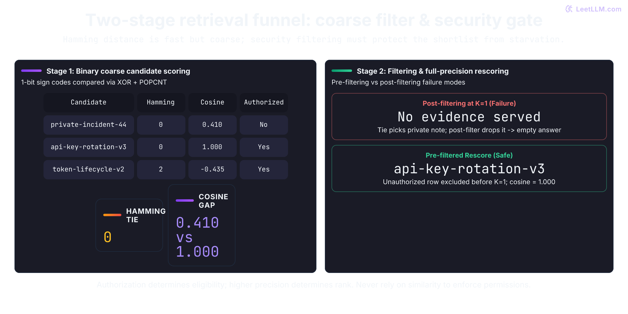
Hamming can tie a private note with the rotation guide. Cosine may separate them, but authorization must work even if the private note has the best possible cosine. The example below compares unfiltered diagnostic shortlists with a permission-filtered search; no private text should reach downstream scoring services.
labels = ["private-incident-note-44", "api-key-rotation-v3", "service-token-lifecycle-v2"]
approved = [False, True, True]
documents = [
    [0.05, -2.00, 0.05, -2.00],  # Same signs, wrong private evidence.
    [0.78, -0.38, 0.58, -0.22],  # Approved rotation guide, close in full precision.
    [0.10, 0.60, -0.40, -0.20],
]
query = [0.80, -0.40, 0.60, -0.20]
expected = "api-key-rotation-v3"

def sign_bits(vector: list[float]) -> list[bool]:
    return [value > 0 for value in vector]

query_signs = sign_bits(query)
hamming = [
    sum(doc_bit != query_bit for doc_bit, query_bit in zip(sign_bits(row), query_signs, strict=True))
    for row in documents
]
unit_query = l2_normalize(query)
def shortlist_at(k: int, *, prefilter: bool) -> list[int]:
    if type(k) is not int or k < 1:
        raise ValueError("shortlist size must be positive")
    candidates = [i for i in range(len(labels)) if not prefilter or approved[i]]
    return sorted(candidates, key=lambda i: (hamming[i], i))[:k]

def serve(shortlist: list[int]) -> str | None:
    allowed = [i for i in shortlist if approved[i]]
    if not allowed:
        return None
    winner = max(allowed, key=lambda i: dot(l2_normalize(documents[i]), unit_query))
    return labels[winner]

shortlist = shortlist_at(2, prefilter=False)
served = serve(shortlist)
assert serve(shortlist_at(1, prefilter=False)) is None
assert serve(shortlist_at(1, prefilter=True)) == expected

recall_at_2 = expected in [labels[index] for index in shortlist]
print(f"binary shortlist={[labels[index] for index in shortlist]}, recall@2={recall_at_2}")
print(f"served evidence={served}, authorized={approved[labels.index(served)]}")
print(f"postfiltered_top1={serve(shortlist_at(1, prefilter=False))}")
print(f"prefiltered_top1={serve(shortlist_at(1, prefilter=True))}")
assert recall_at_2 and served == expectedbinary shortlist=['private-incident-note-44', 'api-key-rotation-v3'], recall@2=True
served evidence=api-key-rotation-v3, authorized=True
postfiltered_top1=None
prefiltered_top1=api-key-rotation-v3At unfiltered K=1, the first-row tie-break chooses the private note and post-filtering returns no evidence. At K=2, the guide survives. Permission filtering before top-K retains the guide even at K=1 in this fixture. On a real ANN index, measure the filtered-search behavior and handle empty results explicitly; increasing K isn't a substitute for access control.
Why is binary quantization usually paired with reranking instead of used as the final answer?
Answer
Binary quantization keeps only one sign bit per dimension, so Hamming distance is fast but coarse. Higher-precision rescoring may improve ordering within the shortlist. Use it, and any optional cross-encoder, when held-out gains justify the cost. It cannot recover missing candidates, and INT8 still approximates the retained FP32 vectors.
Indexing the compressed codes
Compression answers "how many bytes per row?" Approximate Nearest Neighbor (ANN) search answers "how many rows do we visit?" Keep those levers separate. Exact composition is library-specific: some engines combine HNSW graphs with scalar or product quantization, while others keep full-precision vectors beside compressed codes for rescoring.
HNSW (Hierarchical Navigable Small World) organizes vectors into a hierarchy of proximity graphs.[11] Implementations such as hnswlib expose construction and search controls separately.[12]
- Layer 0 (Base layer): Contains every vector in the collection connected by local neighborhood edges.
- Upper layers: Contain nested, exponentially sparser subsets of nodes. One common maximum-level sampler is , with uniform on and . Thus . The fraction retained from one layer to the next is , not . The latter is the exponential scale parameter.[11]
- Search traversal: Search begins at the top layer from a fixed entry point. At each upper layer, search performs a greedy 1-NN walk, hopping along express links until no neighbor is closer to the query than the current node. It then drops to that same node in the layer below and resumes. At Layer 0, the algorithm switches from a greedy 1-NN walk to a prioritized beam search of size to assemble the candidate shortlist.
At , the scale is about 0.289 but only about 3.125% of nodes reach layer 1. Work the probability out before running this analytic calculation; it creates no ANN index:
from math import exp, log

M = 32
level_scale = 1 / log(M)
print(f"M={M}; level_scale={level_scale:.6f}")
for level in (1, 2):
    probability = exp(-level / level_scale)
    print(f"P(max_level >= {level})={probability:.6f}")
assert abs(probability - M ** (-level)) < 1e-15M=32; level_scale=0.288539
P(max_level >= 1)=0.031250
P(max_level >= 2)=0.000977If a compressed index still misses the guide, you need to know which knob can change without rebuilding. HNSW implementations commonly expose three controls:
| Control | Changed during | Systems trade-off | Operational rule |
|---|---|---|---|
| M (connectivity) | Index build | Controls neighbor-link capacity and graph memory. hnswlib estimates roughly – bytes per stored element for this overhead. Actual link counts and representations vary. | Compare rebuilt graphs at fixed queries and search settings; more links cost memory and construction work. |
| ef_construction | Index build | Controls candidate exploration during insertion. More exploration can improve graph quality but lengthens construction; improvements can saturate. | Compare build time, index size, and recall at the intended query budget. No universal build-time complexity follows from one parameter. |
| ef_search | Query serving | Controls the retained nearest-neighbor candidate list. hnswlib requires it to be at least requested ; graph visits are not limited to exactly that many rows. | Measure recall and tail latency together. Lowering it under load can change answer coverage, so keep an explicit quality requirement. |
For scale, an implementation reserving four-byte neighbor IDs at layer 0 uses 256 bytes of neighbor slots when . Counts, upper-layer links, labels, and other structures are extra. That base capacity can exceed a 96-byte PQ code or a 192-byte sign code; it is not the total per-row memory of every HNSW engine.
For example, hnswlib calls the search control ef and sets it with set_ef; its documented search setting must be at least the requested neighbor count. Other engines use names such as efSearch or ef_search.[12]
Start with query-time exploration and measure recall and latency together. If the graph can't reach required recall within the latency budget, rebuild with adjusted construction settings. A copied parameter triple says nothing about a new corpus.
Public benchmarks such as MTEB evaluate embedding models across several task families.[13] They help you assemble candidates. They can't tell you which index retrieves api-key-rotation-v3 under your storage, authorization, and latency limits.
| Decision | Establish a baseline | Accept a change only when |
|---|---|---|
| Model family | Full-precision Recall@K on approved evidence queries | Target slices and latency remain acceptable |
| Supported prefix width | Full trained width with identical scoring | Measured recall loss fits your release threshold |
| SQ, PQ, or BQ | Uncompressed shortlist and final ranking | Compressed shortlist preserves required evidence recall |
| ANN settings | Exact-search results for a labeled sample | Recall and latency both fit the serving budget |
Keep a versioned experiment row for model, width, normalization, quantizer, index settings, shortlist size, and reranker. That row lets you explain a compressed-index rollout when a rotation-guide answer later changes.
Bytes, RAM, and the shortlist bill
The one-million-row example hides scale. Raw float32 payload grows linearly with vector count and can dominate an in-memory index. Disk-backed and hybrid indexes have different memory and I/O tradeoffs; code size alone doesn't establish their latency or total RAM use. The ratios below identify where compression could help.
The byte math is deterministic even when cloud pricing isn't. This table uses the same 1,536-d width as the sizing example, rounded in binary units, before HNSW links, metadata, replicas, or region-specific RAM pricing:
| Scale | Raw payload (1536d, FP32) | With INT8 SQ | With PQ (96-byte code) |
|---|---|---|---|
| 1M vectors | 5.72 GiB | 1.43 GiB | 92 MiB |
| 10M vectors | 57.2 GiB | 14.3 GiB | 916 MiB |
| 100M vectors | 572 GiB | 143 GiB | 8.94 GiB |
| 1B vectors | 5.6 TiB | 1.4 TiB | 89 GiB |
Practice: choose a retrieval stack
You have 50 million API-doc embeddings at 768 dimensions. Some rows, including private-incident-note-44, aren't authorized for this user. P99 latency budget is 60 ms, and raw FP32 vectors would crowd out the rest of the service's RAM. Choose a candidate design to benchmark; the information given can't prove any design meets 60 ms.
- Would you keep raw FP32 payload in memory for first-stage search?
- If your ingest path already L2-normalizes vectors, would you score with cosine or dot product online?
- Would you start with INT8 SQ, PQ, or BQ for the first pass?
- Where would you spend full-precision compute?
- What test prevents a cheaper index from silently changing evidence quality?
Use this as a design review. Give each answer a reason tied to the scoring contract, memory budget, or evidence gate.
Solution sketch:
- FP32 codes require 50M × 768 × 4 = 153.6 GB (about 143.1 GiB). INT8 codes need 38.4 GB; 96-byte PQ codes need 4.8 GB. Add metadata, codebooks, and any retained rescore vectors before comparing RAM budgets.
- Use dot product online if vectors are already unit-normalized. It preserves cosine ranking without redundant norm work.
- Start by benchmarking INT8 SQ because it changes payload less aggressively than PQ or BQ. Move further only when the measured RAM and latency gain justifies shortlist loss.
- Spend full-precision compute on a shortlist, not on the whole corpus. That's where rescoring and reranking pay off.
- Build a labeled release set containing approved rotation and token-lifecycle docs plus tempting unauthorized near-matches. Compare Recall@K with the full-precision baseline, and reject any serving result sourced from unapproved text.
Common pitfalls
When a release goes wrong, the symptom usually points to one boundary. Use it to choose the next measurement instead of changing every knob at once.
- Recall falls after INT8 rollout. Check scale distortion, clipping, omitted scale factors during scoring, and offline/online normalization differences. Compare exact and compressed rankings before changing calibration.
- ANN results look fine offline but wrong in production. Check whether evaluation represents real query language, permissions, and chunking. Inspect misses; a benchmark score alone can't diagnose the cause.
- Search stays slow after quantization. Profile candidate traversal, vector fetches, rescore size, and reranker latency. Tune the expensive stage rather than assuming code payload dominates.
- Migration degrades quality. Check model versions, dimensions, normalization, and quantizer identities. Build the new index separately so incompatible vectors can't silently mix.