Personalize this lesson
Adapt explanations and teaching visuals to your background and preferred voice.
The NumPy lesson tracked what each tensor axis means: examples, token positions, and features. Reuse that shape reasoning for a small access-ticket classifier: four tickets, eight token positions, and 16 features give shape (4, 8, 16). Each ticket is a request that the classifier will label answer, escalate, or block.
Now ask a physical question: where does that same tensor live? An operation can have the right shape and still fail when its tensors disagree about CPU memory versus GPU memory. Follow one miniature batch through indexing, placement, memory pressure, timing, and diagnosis.
CUDA is NVIDIA's platform and programming model for running parallel work on NVIDIA GPUs. It doesn't turn every Python line into GPU code. Python still runs on the CPU, while PyTorch launches GPU functions called CUDA kernels for tensor operations whose data lives on a CUDA device.[1]
If you train on a Mac with Apple silicon, continue through this lesson for the shared accelerator concepts, then use MPS & Metal for ML on Mac for its backend and memory differences.
Eight tokens onto two blocks
Would the four-ticket miniature automatically run faster on a GPU? Not necessarily. A GPU earns its keep when many items perform similar arithmetic; a tiny tensor, branch-heavy Python loop, or copy on every line can lose to launch and transfer overhead.
A CPU is tuned for low-latency control flow and varied work. A GPU is tuned for high throughput. Large matrix multiplications, convolutions, and attention scores usually offer enough parallel arithmetic to justify the handoff.
| Part of a training step | CPU host job | GPU device job |
|---|---|---|
| data preparation | read, tokenize, pad, and assemble a batch | no work yet |
| device transfer | request a copy | receive tensor data in device memory |
| forward and backward | launch PyTorch operations | execute tensor kernels |
| reporting | request a Python number or file write | finish and return needed values |
The CPU prepares and launches; the GPU executes. Inside one kernel launch, a thread handles one logical slice of work. Threads are grouped into thread blocks, and all blocks for one kernel form a grid. CUDA schedules each whole block onto one streaming multiprocessor (SM), a hardware processor inside the GPU. Several blocks may be active on one SM, and CUDA doesn't promise which block runs first.[1]
Take just the eight token positions of the first ticket, not all four tickets or all their features. Two blocks with four threads each is a convenient teaching size. Before running the trace, predict which block and thread own T6. For a one-dimensional grid of one-dimensional blocks, each thread computes a unique global index:
For block 1, thread 2, the global index is 1 × 4 + 2 = 6, so that thread handles token position T6. The Python trace checks all eight assignments before the CUDA vocabulary grows. It takes block and thread counts as input and prints each block's token positions:
1threads_per_block = 4
2blocks = 2
3
4for block_id in range(blocks):
5    positions = []
6    for thread_id in range(threads_per_block):
7        global_id = block_id * threads_per_block + thread_id
8        positions.append(f"T{global_id}")
9 print(f"block {block_id}: {positions}")1block 0: ['T0', 'T1', 'T2', 'T3']
2block 1: ['T4', 'T5', 'T6', 'T7']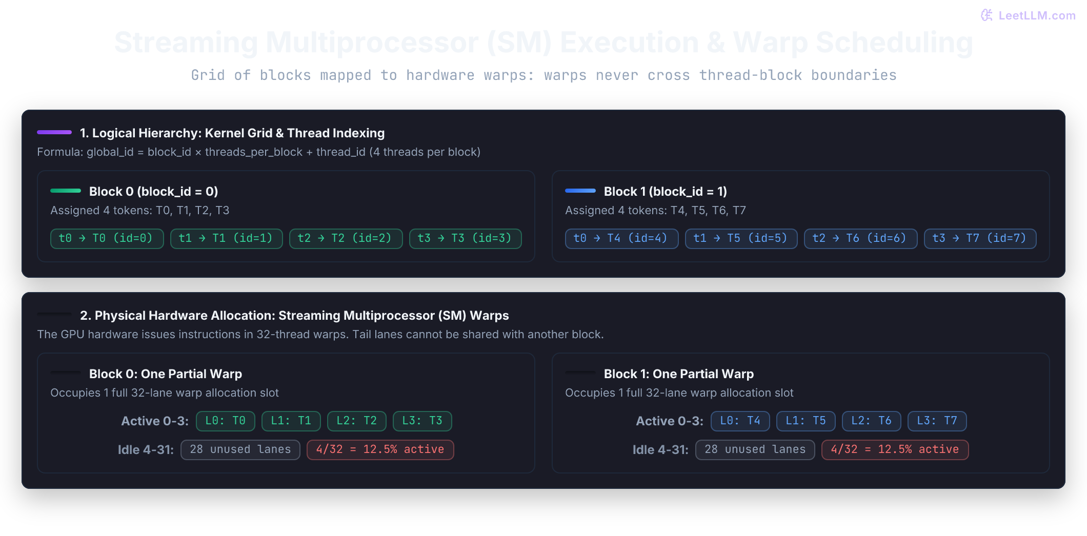
The trace has eight useful threads, but hardware groups threads into a larger unit. An NVIDIA CUDA warp contains 32 threads from one block. Warp lanes execute through a single-instruction, multiple-thread (SIMT) model. If lanes take different branches, CUDA masks inactive lanes while it executes each required path, so divergence can waste throughput.[1]
The four-thread teaching block is legal, and it still occupies a full warp. CUDA fills that warp with consecutive thread ids from the same block, so 4 lanes do ticket work and 28 lanes sit unused for the whole launch. That's a teaching cost, not a production default.
Read the hierarchy from a kernel launch downward: its grid contains blocks; each block is scheduled on one SM and advances in warps; each thread owns its index. A PyTorch operation can launch several kernels, and a shape-only view can launch none. Use the table to name what each level contributes:
| Level | Meaning | Beginner question |
|---|---|---|
| PyTorch operation | a request such as x * 2 or x @ w | Is the tensor on CUDA? |
| kernel | GPU function launched to perform part of the work | Is the work large enough to justify a launch? |
| grid | every block in one launch | How much work exists? |
| block | threads that run on one SM and can cooperate | Which slice of work stays together? |
| warp | 32 threads scheduled together | Are branches, or a short last warp, leaving lanes idle? |
| thread | one logical worker with its own index | Which data item does it handle? |
PyTorch's matrix-multiply kernels use optimized tiling that is more complex than one thread per token. The eight-position trace teaches indexing and scheduling vocabulary without pretending to describe an optimized library kernel exactly.
What if there are ten positions instead of eight? Two four-thread blocks miss the last two positions; three blocks create twelve threads. The final two threads need a bounds check before reading or writing an array. This CPU simulation checks both coverage and the unused tail:
1positions = 10
2threads_per_block = 4
3blocks = (positions + threads_per_block - 1) // threads_per_block
4visited = []
5skipped = []
6for block_id in range(blocks):
7    for thread_id in range(threads_per_block):
8        i = block_id * threads_per_block + thread_id
9        if i < positions:
10            visited.append(i)
11        else:
12            skipped.append(i)
13assert visited == list(range(positions))
14print("blocks:", blocks)
15print("guarded indexes:", skipped)1blocks: 3
2guarded indexes: [10, 11]Removing the guard would attempt indexes 10 and 11, beyond the ten-element array. These are ordinary Python simulations of CUDA indexing, not GPU kernels. PyTorch supplies the indexing and bounds handling for the tensor operations used below.
Those launches only happen if this process can see a CUDA device. The next check is whether the driver, the PyTorch build, and the GPU agree.
Check driver, PyTorch build, and device
The phrase "my CUDA version" hides several boundaries. Before running any command, predict what each tool can actually prove. The NVIDIA System Management Interface command, nvidia-smi, reads driver and GPU state; nvcc is NVIDIA's CUDA compiler:
| Signal | What it tells you | What it doesn't prove |
|---|---|---|
nvidia-smi | NVIDIA driver can see a GPU. The CUDA Version header (documented as CUDA UMD Version; the older CUDA Version label is deprecated) is the latest CUDA version that driver supports | which CUDA toolkit is installed, or whether this Python has a CUDA-enabled PyTorch build |
torch.__version__ | installed PyTorch version and often its build suffix | whether GPU access works |
torch.version.cuda | CUDA version used to build this PyTorch package, or None for a build without CUDA | whether driver and device are reachable |
torch.cuda.is_available() | CUDA is currently available to this process | whether a particular kernel can execute, fits, or runs fast |
nvcc --version | version of local CUDA toolkit compiler, when installed | which runtime a prebuilt PyTorch package uses |
The CUDA UMD Version describes driver capability, not an installed compiler. A machine can run a prebuilt CUDA-enabled PyTorch package without having nvcc installed.[2] It can't prove that this Python process loaded a CUDA-enabled PyTorch build.
PyTorch's installer offers builds for supported compute platforms, and its verification step uses torch.cuda.is_available().[3] For ordinary prebuilt use, a local toolkit and nvcc matter when you build PyTorch from source or compile custom CUDA extensions. Version strings don't need to match; the driver must support the runtime used by the package.
Run the driver check first, then inspect the Python environment. The shell command produces driver output, PyTorch version and runtime, availability, device name, capability, and architectures when CUDA is reachable:
1nvidia-smi
2python3 - <<'PY'
3import torch
4
5print("PyTorch:", torch.__version__)
6print("PyTorch CUDA runtime:", torch.version.cuda)
7print("CUDA available:", torch.cuda.is_available())
8
9if torch.cuda.is_available():
10    print("device:", torch.cuda.get_device_name(0))
11    print("compute capability:", torch.cuda.get_device_capability(0))
12    print("build architectures:", torch.cuda.get_arch_list())
13PY
The compute capability pair describes hardware features supported by a GPU generation. get_arch_list() reports architectures included in the PyTorch build. Read the first disagreement, not the most alarming line:
| Observed state | Likely boundary | Next check |
|---|---|---|
nvidia-smi fails | driver, hardware, or container access | driver installation and device exposure |
nvidia-smi works, torch.version.cuda is None | PyTorch package wasn't built for CUDA | select the CUDA-enabled package for this environment |
PyTorch has a CUDA runtime, but availability is False | driver compatibility or process visibility | driver support, container GPU access, CUDA_VISIBLE_DEVICES |
availability is True, but kernel reports unsupported architecture | installed binary doesn't support this GPU | check support in PyTorch and any custom extension; older GPUs can also lose support |
availability is True and device name is correct | basic stack works | test placement, memory, and timing |
CUDA_VISIBLE_DEVICES changes the GPU indexes visible inside the process. If physical GPU 1 is the only visible device, PyTorch may call it cuda:0. Inspect tensor.device and device names inside the running process instead of assuming host indexes survive a mask.
Once the stack answers "yes," the miniature ticket batch still has to move. A visible GPU is only permission to try work; it isn't proof that tensors, memory, or timing are correct.
Move the ticket batch once
Return to the (4, 8, 16) ticket tensor. What changes during .to(device): its shape or its residence? Shape stays constant; residence changes from host memory to CUDA device memory.
On a discrete NVIDIA GPU, a host-to-device (H2D) transfer copies data from CPU memory to GPU memory. Device-to-host (D2H) is the return path. Keep model weights, batch tensors, activations, gradients, and optimizer state on the GPU through the hot part of a training step. Bring back the small value needed for reporting.
The runnable step uses random feature values so it needs no dataset download. It tests execution, not classifier quality. It averages eight token vectors into one vector per ticket, then scores three classes. Labels are 0 = answer, 1 = escalate, 2 = block.
nn.Linear(16, 3) multiplies each 16-feature vector by learned weights and adds a bias, producing three scores called logits. Cross-entropy turns those scores and the correct label into one error value, the loss. backward() computes how each weight affects that loss; those derivatives are gradients. Stochastic gradient descent (SGD) updates weights opposite the gradient, aiming to reduce the loss.[4] The later PyTorch training lesson derives the loop; here, watch where its tensors live.
Predict its shape and device checks before running: (4, 8, 16) should become ticket vectors (4, 16) and logits (4, 3). On CUDA, model and batch should agree; on CPU, the same shape and loss checks still run.
1import math
2
3import torch
4import torch.nn as nn
5import torch.nn.functional as F
6
7torch.manual_seed(7)
8device = torch.device("cuda:0" if torch.cuda.is_available() else "cpu")
9
10model = nn.Linear(16, 3).to(device)
11optimizer = torch.optim.SGD(model.parameters(), lr=0.1)
12
13cpu_batch = {
14    "token_features": torch.randn(4, 8, 16),
15    "labels": torch.tensor([0, 2, 1, 0]),
16}
17batch = {name: tensor.to(device) for name, tensor in cpu_batch.items()}
18
19optimizer.zero_grad()
20ticket_vectors = batch["token_features"].mean(dim=1)
21logits = model(ticket_vectors)
22loss = F.cross_entropy(logits, batch["labels"])
23loss.backward()
24optimizer.step()
25
26model_device = next(model.parameters()).device
27assert all(tensor.device == model_device for tensor in batch.values())
28assert logits.device == loss.device == model_device
29assert ticket_vectors.shape == (4, 16) and logits.shape == (4, 3)
30reported_loss = loss.detach().cpu().item()
31print("selected accelerator:", device.type == "cuda")
32print("model and batch agree:", model_device == batch["token_features"].device)
33print("ticket vectors:", tuple(ticket_vectors.shape))
34print("logits:", tuple(logits.shape))
35print("finite loss:", math.isfinite(reported_loss))
On an accessible NVIDIA GPU, the first two lines should report True. A CPU-only machine reports False for the accelerator line but still validates tensor and training logic. If a shape fails, debug the reduction or linear layer first; a device error needs a different branch.
Device placement applies to every tensor an operation touches. Moving features but leaving labels on CPU still fails during a CUDA loss calculation. Deliberately leave the features on CPU in the next fragment. Predict the error on a CUDA machine, and the fallback message on a CPU-only machine:
1import torch
2import torch.nn as nn
3
4if torch.cuda.is_available():
5    cuda_model = nn.Linear(16, 3).to("cuda")
6    cpu_features = torch.randn(4, 16)
7    try:
8        cuda_model(cpu_features)
9    except RuntimeError as error:
10        if "device" not in str(error).lower():
11            raise
12        print("device mismatch:", str(error))
13    else:
14        raise AssertionError("expected a mixed-device forward pass to fail")
15else:
16    print("CUDA unavailable: real mixed-device failure wasn't executed")
The symptom is an error saying tensors or arguments aren't on the same device. Cause is placement, not shape. Move every participating tensor to the model's device before the forward or loss call. Synchronizing won't repair a tensor stored on the wrong device.
The miniature step can succeed while a training-sized batch still fails. Shapes and device placement answer whether an operation is legal; memory pressure decides whether the full forward and backward pass can coexist.
Count memory before the first big batch
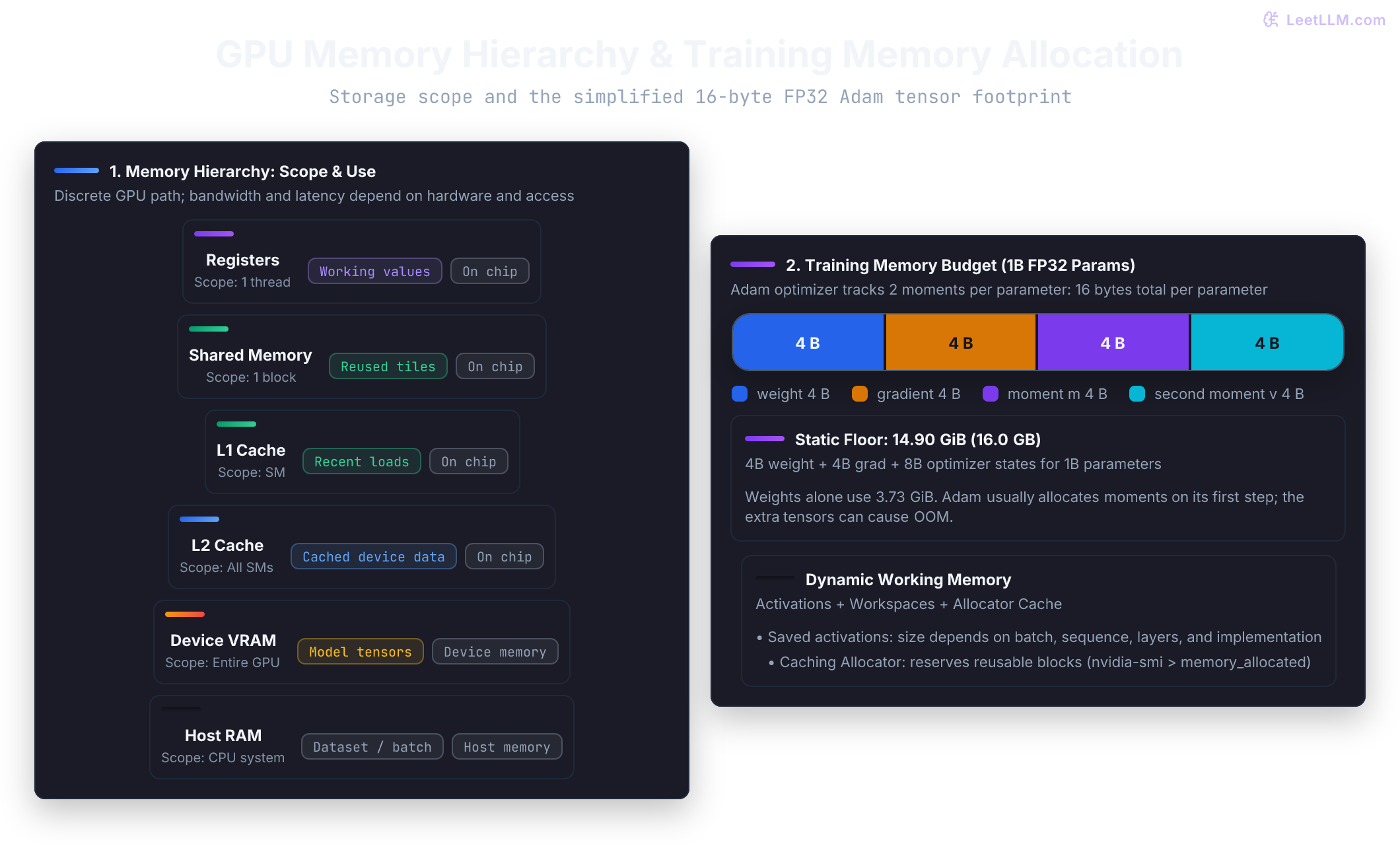
The small step fits. Before increasing batch size, ask which values must survive between steps and which exist only while one kernel runs. CUDA exposes several storage levels, and they aren't interchangeable:
| Storage | Scope | Typical training data |
|---|---|---|
| host RAM | CPU process | dataset objects, decoded examples, CPU batches |
| device global memory, often called video RAM (VRAM) or high-bandwidth memory (HBM) | all SMs on one GPU | weights, activations, gradients, optimizer state |
| L2 and L1 caches | GPU hardware | recently accessed device data |
| shared memory | threads in one block | tiles reused inside a kernel |
| registers | one thread | counters, addresses, and small working values |
PyTorch allocates model tensors in device global memory. Optimized kernels decide when to reuse tiles through caches, shared memory, or registers. Calling .to("cuda") doesn't place a whole tensor in a register or in shared memory. An optimizer adds its own long-lived state during training.
The miniature batch itself contains 4 × 8 × 16 = 512 float32 values, only 2,048 bytes. A larger (32, 128, 768) float32 batch contains 32 × 128 × 768 × 4 = 12,582,912 bytes, exactly 12.0 MiB of input features. That input is only one term in a training step:
The example uses SGD without momentum, which doesn't keep per-parameter running statistics. To see why the optimizer choice changes memory, consider Adam, an optimizer that tracks two statistics for each parameter: a running average of gradients and a running average of squared gradients.[5]
For a simplified full-precision Adam budget, count 4 bytes for each weight, 4 for its gradient, and 8 for its two statistics. One billion parameters therefore require 16 billion bytes for these tensors when they're all present. Activations, temporary buffers, allocator overhead, and any extra parameter copies still sit outside this accounting.
Compute those two scales before touching a GPU. The first value is a batch input; the second is a parameter-related floor. The script takes the parameter count and feature shape as constants and prints both in human-readable units:
1parameters = 1_000_000_000
2bytes_per_parameter = 4 + 4 + 8
3total_bytes = parameters * bytes_per_parameter
4feature_bytes = 32 * 128 * 768 * 4
5
6print(f"bytes per parameter: {bytes_per_parameter}")
7print(f"parameter-related floor: {total_bytes / (1024 ** 3):.2f} GiB")
8print(f"training-sized ticket features: {feature_bytes / (1024 ** 2):.1f} MiB")
9print("activations and temporary work: add more memory")1bytes per parameter: 16
2parameter-related floor: 14.90 GiB
3training-sized ticket features: 12.0 MiB
4activations and temporary work: add more memoryA model can load and still hit an out-of-memory (OOM) failure on its first forward or backward pass. Loading proves that current state fits. It doesn't prove that activations and gradients for a real batch fit. Adam's moment tensors are commonly created on the first optimizer step, so that step can fail even after backward succeeds.
For the running text batch, predict which change halves token positions: halve batch size, or halve sequence length? Both halve the simple B × T count, but attention storage responds differently. This small calculation makes that distinction visible:
1batch_size = 32
2sequence_length = 128
3baseline = batch_size * sequence_length
4
5for name, batch, tokens in [
6    ("baseline", 32, 128),
7    ("half batch", 16, 128),
8    ("half length", 32, 64),
9]:
10    share = batch * tokens / baseline
11 print(f"{name:11s}: {share:.0%} of token positions")1baseline : 100% of token positions
2half batch : 50% of token positions
3half length: 50% of token positionsThe output counts token positions, not full memory. Our mean-pooling classifier has no attention matrix. A later transformer compares each token with every other token; storing those scores can require a tensor shaped (B, H, T, T), where B is batch size, H is the number of attention heads, and T is sequence length. Halving B halves that tensor; halving T quarters it. Memory-efficient attention can avoid storing the full score matrix, so this isn't a universal prediction of peak memory. Feature width D = 768 doesn't change the token-position count.
Mixed precision is another memory and throughput tool, but it isn't a safe synonym for calling .half() on everything. PyTorch's automatic mixed precision (AMP) uses torch.autocast(device_type="cuda") to choose an operation-specific dtype. FP16 (16-bit floating point) training may need torch.amp.GradScaler("cuda") to prevent small gradients from underflowing, and some models overflow in FP16.[6] Confirm finite loss, finite gradients, and expected model quality. The dedicated mixed-precision lesson covers that workflow.
TensorFloat-32 (TF32) is a separate choice on Ampere and newer NVIDIA GPUs: eligible operations keep float32 tensor storage but use reduced-precision inputs internally, with FP32 accumulation. It can change numerical results without halving tensor memory. Current PyTorch documentation recommends fp32_precision controls such as torch.backends.cuda.matmul.fp32_precision = "ieee" or "tf32"; mixing these with legacy allow_tf32 controls isn't supported. Record the precision setting when comparing timings, and check accuracy before accepting a faster setting.[7]
Memory pressure answers "does it fit?" It doesn't answer whether the GPU is moving data efficiently while it works. Access order supplies that missing piece.
Let access order decide bandwidth
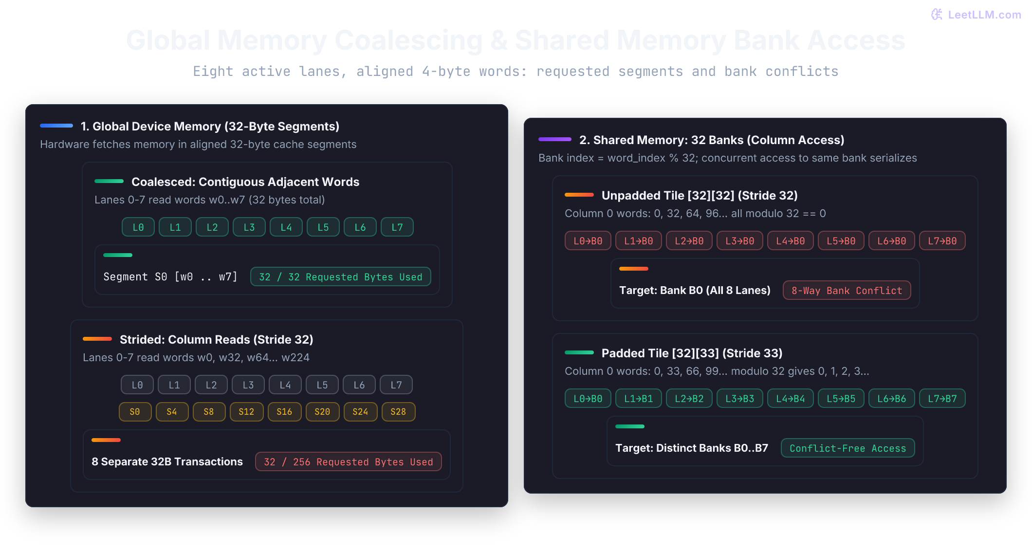
Two kernels can read the same number of float32 values and still ask the memory system for very different work. On GPUs with compute capability 6.0 or newer, a warp's global-memory requests are serviced in 32-byte segments. Reading adjacent words lets the lanes share segments, an access pattern called coalescing. Reading a column in a row-major matrix can instead make neighboring lanes jump by a stride of 32 words, so each lane touches a different segment.
Keep eight lanes in the illustration so the addresses stay readable. For a full warp, the adjacent pattern needs four 32-byte transactions when the first word is aligned. The stride-32 pattern can need one transaction per lane. That's why a mathematically identical operation can land on opposite sides of a bandwidth limit.[8]
Shared memory can repair the global access pattern, but it introduces banks, independently accessible storage partitions. In the standard 32-bank layout for 32-bit words, the bank index is the word index modulo 32. For column zero of a 32 × 32 tile, lanes 0, 1, and 2 access word indexes 0, 32, and 64, all in bank 0. These are different addresses, so the accesses serialize. With a 32 × 33 allocation, the indexes become 0, 33, and 66, which map to banks 0, 1, and 2. Padding changes storage layout, not the logical matrix result. Multiple lanes reading the same address are a broadcast case, not this bank-conflict case.[8]
Use this compact table after you've inspected the access pattern. It names the first change worth testing, not a promise that one trick wins every kernel:
| Observed access | What the hardware sees | First experiment |
|---|---|---|
| adjacent global words | a few 32-byte transactions | keep the layout and measure another bottleneck |
| strided global words | many transactions for the same useful values | load coalesced rows, then reorder in shared memory |
| shared tile stride 32 | several lanes contend for one bank | add a padding column and remeasure |
| shared tile stride 33 | lanes spread across banks | keep padding only if output and end-to-end time improve |
The table explains why "put it in shared memory" isn't a complete optimization. Shared memory helps when it removes global traffic or fixes an access pattern; bank conflicts can give that shortcut a new bottleneck.[8]
Memory layout answers where time can go. The next question is whether arithmetic or bytes set the upper bound.
Choose the next optimization with a bound
Suppose a kernel performs 1,000 floating-point operations (FLOPs) and transfers 4,000 bytes to or from device memory. That's 0.25 FLOPs/byte: little arithmetic for each byte fetched. This ratio is called arithmetic intensity:
Double the bytes without changing the math and intensity falls to 0.125. The Roofline performance model combines this ratio with two hardware limits: arithmetic per second and bytes per second. Its upper bound is the smaller of the compute ceiling and bandwidth multiplied by intensity. Count bytes and bandwidth at the same memory level; a device-memory Roofline uses traffic beyond the caches, not every load instruction.[9][10]
For a hypothetical device with a 100 GFLOP/s compute ceiling and 40 GB/s memory bandwidth, intensity 0.25 gives a bandwidth ceiling of 40 × 0.25 = 10 GFLOP/s. The bound is therefore 10, not 100 GFLOP/s. These invented numbers teach the units; they aren't a GPU benchmark.
Predict before tuning: when intensity is low and measured bandwidth is high, will adding more arithmetic make the kernel faster? Usually not. Reuse data, reduce bytes, or make requests coalesced first. When intensity is high but achieved floating-point rate stays far below the compute ceiling, inspect instruction choice, layout, and launch resources instead.
Occupancy is the fraction of an SM's maximum resident warps that are currently resident. A resident warp holds execution resources even while waiting for data. Having other ready warps helps the scheduler hide that wait, but 100% occupancy isn't a target by itself. Registers and shared memory are finite; using more of either can reduce the number of resident blocks. A kernel with lower occupancy can still win if its tiles reuse data or its threads do more useful work. Treat occupancy as a constraint and a clue, then let measured throughput and stall reasons decide.[8]
NVIDIA's Assess, Parallelize, Optimize, Deploy (APOD) cycle gives the work a safe rhythm. At this level, combine its Parallelize and Optimize stages into one controlled change:
- Measure (Assess): profile a representative shape and record end-to-end time, kernel time, output, and memory behavior.
- Change (Parallelize, then Optimize): alter access order, reuse, dtype, launch shape, or transfer behavior because the evidence points there.
- Verify, Deploy, and repeat: compare output with a trusted reference, rerun the same measurement, keep the change only when the whole step improves, then start the next pass from a fresh assessment.
Pick the tool from the question. Nsight Systems answers whether the CPU feeds the GPU and where transfers, kernels, streams, or host waits leave gaps. Nsight Compute answers what one kernel does with its launch resources, memory hierarchy, and compute or bandwidth ceilings. Compute Sanitizer answers whether custom CUDA work reads or writes illegal memory, races on shared memory, or violates synchronization. A speedup without the last check is only a faster way to trust a bad result.[11][10][12]
| Question | First tool | Evidence to read |
|---|---|---|
| Is the step CPU-, transfer-, or synchronization-bound? | Nsight Systems (nsys profile --trace=cuda) | CUDA API and GPU workload timelines, H2D copies, kernels, streams, and idle gaps |
| Is one kernel limited by bytes, math, or launch resources? | Nsight Compute (ncu) | launch statistics, SpeedOfLight, Roofline, cache traffic, bank conflicts, and warp stalls |
| Did a custom kernel produce invalid work? | Compute Sanitizer | memcheck, racecheck, and synccheck reports with source, block, and thread context |
Run correctness checks before comparing numbers. Once the bound and the failure surface are named, the diagnosis table can point to a narrow next action instead of turning every slowdown into a memory tweak.
CUDA's default async launch makes timing another boundary that is easy to get wrong.
Measure asynchronous work honestly
PyTorch queues CUDA operations asynchronously by default. The CPU can finish a Python call while its GPU kernels are still waiting or running. Operations in the same CUDA stream keep their order, so later GPU work sees correct results without a host wait. A host-visible value or explicit synchronization makes the CPU wait.[7]
Suppose a larger classifier's forward pass takes 40 ms on the GPU, while Python needs only 2 ms to queue it. These are illustrative numbers, not measurements of our miniature classifier. Predict what a host timer around the call reports: it measures the caller's elapsed time, not necessarily completed device work.
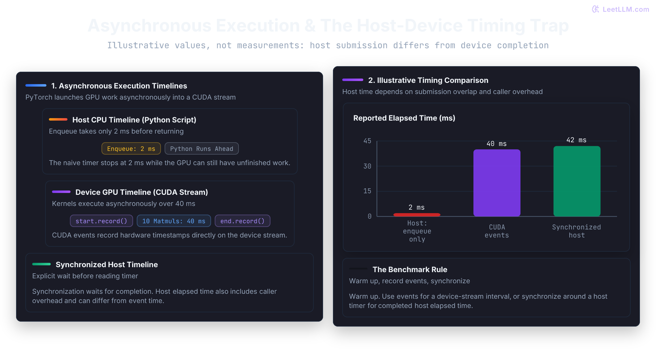
The naive timer stops at 2 ms while the GPU continues. Events record timestamps on a CUDA stream, an ordered queue of device work. Their interval includes work and any gaps between the events on that stream; it isn't automatically the sum of individual kernel durations. A synchronized host timer can also include Python overhead, so it needn't match event time exactly.
Warm up first because initial calls may include library setup or kernel selection. This script times ten matrix multiplications with CUDA events, or a host timer on CPU, and checks the result against a CPU reference. The timed region excludes input allocation, warmup, transfers, and the correctness check:
1import time
2
3import torch
4
5device = torch.device("cuda:0" if torch.cuda.is_available() else "cpu")
6x_cpu = torch.arange(256 * 256, dtype=torch.float32).reshape(256, 256) % 8
7x = x_cpu.to(device)
8
9for _ in range(3):
10    result = x @ x
11
12if device.type == "cuda":
13    torch.cuda.synchronize()
14    start = torch.cuda.Event(enable_timing=True)
15    end = torch.cuda.Event(enable_timing=True)
16    start.record()
17    for _ in range(10):
18        result = x @ x
19    end.record()
20    torch.cuda.synchronize()
21    elapsed_ms = start.elapsed_time(end)
22else:
23    start_time = time.perf_counter()
24    for _ in range(10):
25        result = x @ x
26    elapsed_ms = (time.perf_counter() - start_time) * 1000
27
28torch.testing.assert_close(result.cpu(), x_cpu @ x_cpu, rtol=1e-4, atol=1e-4)
29print("timing backend:", device.type)
30print("result shape:", tuple(result.shape))
31print(f"mean completed matmul: {elapsed_ms / 10:.3f} ms")
32print("completed timing is positive:", elapsed_ms > 0)
Common host waits include:
loss.item()for a Python scalartensor.cpu()before CPU analysistensor.cpu().numpy()before NumPy work- printing a CUDA tensor's values
torch.cuda.synchronize()
Those operations aren't bugs. They become performance bugs when they sit inside a hot loop more often than reporting or correctness requires. A scalar needed once per full pass is different from a scalar pulled back every step.
Asynchrony also affects error location. A bad kernel may report its error on a later Python line that finally waits for the device. For one debugging reproduction, run with CUDA_LAUNCH_BLOCKING=1 to make CUDA calls synchronous and recover a more useful stack trace. Remove it before performance measurement because it changes execution behavior.[7]
When the ticket step is slow, empty, or dead, start with one question: did the CPU fail to feed the GPU, did the GPU run work that doesn't fit, or did the measurement hide the wait? The diagnosis table turns that question into first actions.
Diagnose setup, memory, and throughput failures
nvidia-smi is a useful first observation, not a kernel profiler. Use it to confirm device visibility, process attachment, rough memory pressure, and utilization samples. Before comparing its memory number with PyTorch, predict which one includes reserved-but-unused allocator blocks. PyTorch's caching allocator can hold blocks for reuse, so nvidia-smi may show more memory than live tensors occupy.[2][7]
PyTorch separates two allocator views:
torch.cuda.memory_allocated()counts memory occupied by live tensors.torch.cuda.memory_reserved()counts the larger pool managed by PyTorch's caching allocator.
torch.cuda.empty_cache() releases unused cached blocks for other applications. It doesn't free live tensors or shrink the workload's required memory. Cached blocks are normally reusable by the same job already; repeatedly clearing them can add allocation overhead. nvidia-smi also includes CUDA context and other allocations outside PyTorch's tensor allocator, so it needn't equal memory_reserved().[7]
Use symptom, cause, and next action together. Choose the first row that matches observed evidence instead of tuning every knob at once:
| Symptom | Likely cause | First action |
|---|---|---|
torch.cuda.is_available() is False | driver, visibility, or PyTorch build mismatch | compare nvidia-smi, torch.version.cuda, and process visibility |
| forward says tensors are on different devices | model and one batch field disagree | move every tensor used by model or loss to model device |
| model loads, backward OOMs | activations, gradients, optimizer state, or workspace exceed free memory | lower per-step batch size, then sequence length; read allocation size in OOM message |
| effective batch must stay large | smaller steps change optimization batch | accumulate gradients across several smaller steps and scale loss correctly |
loss or gradients become not-a-number (NaN) under FP16 | numerical overflow or invalid mixed-precision path | disable AMP to reproduce, then use autocast and scaling with finite-value checks |
| host timer says a kernel took almost zero time | CPU timed enqueue only | warm up and use CUDA events or explicit synchronization |
| memory bar is high but examples per second are low | allocation isn't utilization; data, copies, sync, or tiny kernels may stall | inspect dataloading and host waits before blaming matrix kernels |
| GPU utilization repeatedly falls to zero | possible input starvation, host waits, or brief work missed by sampling | profile data loading, transfer cadence, and synchronization gaps |
| CUDA error points at an innocent later line | asynchronous error surfaced at next wait | reproduce once with CUDA_LAUNCH_BLOCKING=1 |
Pinned host memory can speed H2D copies. DataLoader(..., pin_memory=True) prepares CPU tensors in page-locked memory, and .to(device, non_blocking=True) can let the host continue without waiting for each transfer. This doesn't by itself overlap the copy with a later kernel in the same stream: their order is preserved. Actual copy/compute overlap requires suitable hardware, separate streams, and correct dependencies. Don't modify a pinned source buffer until its asynchronous copy finishes.[13]
The next snippet is a transfer-boundary fragment, not a full script. It assumes a CPU dataset yielding (features, labels) and a model already exist. Deriving the device from the model gives an explicit index such as cuda:0, not an unindexed cuda specification:
1from torch.utils.data import DataLoader
2
3device = next(model.parameters()).device
4loader = DataLoader(dataset, batch_size=32, pin_memory=(device.type == "cuda"))
5
6for features, labels in loader:
7    features = features.to(device, non_blocking=True)
8    labels = labels.to(device, non_blocking=True)
9    assert features.device == device and labels.device == device
10    # Forward, backward, and optimizer work stay on device.
Measure before and after. Pinned memory and non-blocking copies help a transfer bottleneck; they won't fix a kernel that's already compute-bound or an OOM caused by live tensors. A faster copy doesn't change the amount of model state that must fit.
Trace the training step end-to-end
Use the complete training step as a small accelerator artifact. A note saying "GPU works" collapses setup, shape, placement, memory, and timing into one unverifiable claim. Record one piece of evidence for each boundary.
- Predict shapes before running: batch
(4, 8, 16), pooled vectors(4, 16), logits(4, 3). - Run
nvidia-smiand the PyTorch environment check. Record driver, PyTorch runtime, device name, and availability separately. - Run the training step. Confirm model, features, labels, logits, and loss use one device until reporting.
- Deliberately leave features on CPU while model is on CUDA. Capture the device-mismatch symptom, then restore
.to(device). - Time ten matrix multiplies with CUDA events. Compare that result with a naive host timer around the same loop.
- Write the terms that would make a larger run OOM: weights, activations, gradients, optimizer state, workspaces, and allocator overhead.
Compare expected output with this table, then correct the first boundary that fails. A later symptom can be downstream noise:
| Evidence | Pass condition | If it fails |
|---|---|---|
| shape trace | (4, 8, 16) → (4, 16) → (4, 3) | revisit reduction axis or linear-layer input width |
| device trace | every training tensor matches model device | move missing batch field before operation that uses it |
| timing trace | event reports completed GPU work | add warmup and synchronization after end event |
| memory trace | full training footprint is named | add activations, gradients, optimizer state, and temporary work |
Check the reasoning without running code. Each answer should name a mechanism, not only repeat a command:
Why can model(x) return to Python before its CUDA kernels finish?
Answer
PyTorch queues CUDA work asynchronously. Python can continue after enqueueing while the device executes operations in stream order.
Why can a model fit in device memory and then OOM during backward?
Answer
Model loading accounts for current state, but training also needs activations, gradients, optimizer state, temporary workspaces, and allocator overhead.
Why can nvidia-smi show more memory than memory_allocated()?
Answer
PyTorch's caching allocator can reserve unused blocks for fast reuse. memory_allocated() counts live tensors, while nvidia-smi can reflect the larger reserved pool.
What does the CUDA value printed by nvidia-smi mean?
Answer
It's the latest CUDA version the installed driver supports (CUDA UMD Version; the older CUDA Version label is deprecated). It isn't proof that the same toolkit is installed or that this PyTorch environment can use CUDA.
Carry shape, device, and timing forward
A CUDA training step has three contracts:
- Shape: each axis still means what the model expects.
- Device: every tensor used together lives on a compatible device.
- Time: measurements include the GPU work whose latency you intend to report.
The CPU prepares data and launches work. CUDA maps kernels onto grids, blocks, warps, and SMs. Device memory holds long-lived training state, while kernels use caches, shared memory, and registers for smaller working sets. Copies and synchronization are explicit costs, so placement, OOM diagnosis, and timing all follow from the same execution path.
If a run fails, ask which contract broke first: shape, device, or time. That question narrows a large CUDA surface into an observable next check.
The Mac lesson keeps those checks but changes the hardware picture: Apple silicon doesn't give you a separate VRAM pool copied over PCIe.