Personalize this lesson
Adapt explanations and teaching visuals to your background and preferred voice.
At 09:00, a cluster scheduler has to decide whether to intervene before a training job misses its SLA (service-level agreement). The queue worker knows the input size, heartbeat age, backlog depth, and priority tier. The true label arrives hours later, once the worker finishes or times out. Historical records can train a model, but an upcoming job still needs a score and a concrete rule that translates that score into an operational action.
A gradient-boosted tree is a useful tabular baseline. Grinsztajn et al.'s 2022 benchmark found strong tree results on its medium-sized datasets, around 10,000 rows; that isn't a permanent ranking of all tabular methods.[1] Later work, including TabPFN's 2025 study, demonstrates competitive neural foundation models in a defined small-data regime.[2] This lesson asks a narrower question: can a booster justify its maintenance cost against cheap alerting policies?
Each new tree fits a correction based on the current loss gradient. We'll inspect one correction, choose rounds and thresholds on later jobs, and keep the evidence separate from permission to operate the service.
Freeze the clock before training
Suppose missed_sla = 1 indicates that a training run blew past its promised completion window. Before fitting an ensemble, answer one foundational question: which rows and features were genuinely available when each historical decision occurred? A time-ordered split makes that boundary explicit:
| Split | Calendar range | Operational role |
|---|---|---|
| train | January through March | fit tree ensemble weights and splits |
| validation | April | select round count, stopping point, and operating threshold |
| test | May | evaluate frozen candidate on unseen future traffic |
A random shuffle can spread one cluster disruption across fitting and holdout rows, making evidence optimistic for a future-incident deployment. Chronological evaluation matches that target, but dates alone don't enforce feature availability or incident separation. If an incident straddles a cutoff, explicitly purge or assign its linked rows while preserving the intended time boundary. A random split can still suit a different, exchangeable prediction population.
Point-in-time correctness extends to every individual feature. Official guidance warns against training on information unavailable at scoring time.[3] A feature recorded after the dispatch timestamp represents feature leakage, even if the column appears innocuous. Labels obey availability clocks as well: a March job still running on April 1 can't feed its final outcome into an April 1 retraining run.
Missing-value support depends on the estimator. XGBoost learns default routing during sparsity-aware split search.[4] Scikit-learn's HistGradientBoostingClassifier learns routing too; if a feature had no missing training values, it sends a prediction-time NaN to the child with more samples. That fallback is deterministic, not arbitrary.[5] The classic GradientBoostingClassifier used in this lab rejects NaNs in the checked environment.
Native routing doesn't validate a new telemetry outage. Test missingness patterns against the serving contract, and keep any imputer fitted on training rows only. Unknown categorical values are a separate contract.
Read the evaluation flow below as a sequence of strict gates. April freezes the hyperparameters and the operational threshold; May scores the candidate exactly once. Passing metric checks triggers operational review rather than authorizing immediate automated release.
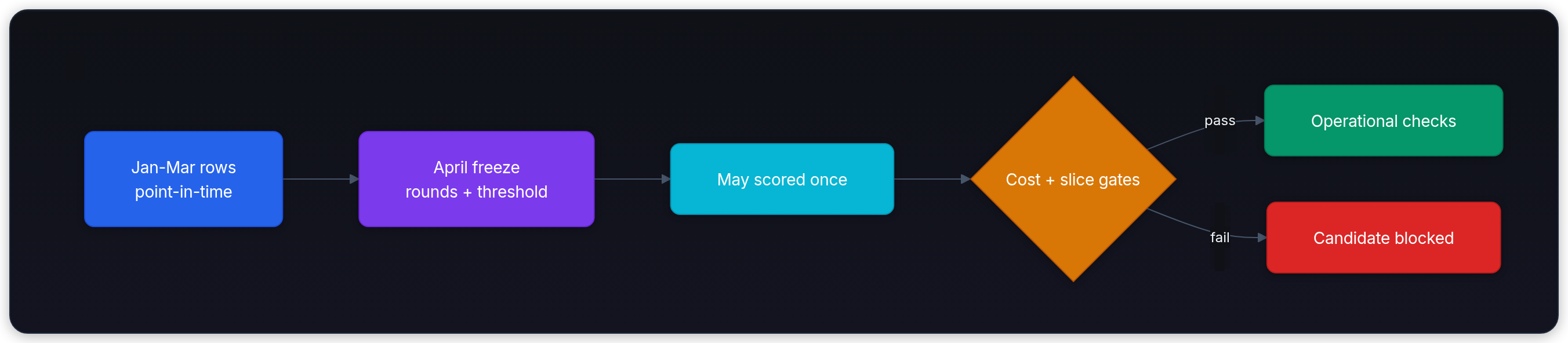
Build a seeded synthetic fixture with three month-labelled groups. It assumes every feature and training label meets the timing contract; it doesn't implement timestamp joins or incident grouping. Labels depend on heartbeat age, backlog, priority, and a large-model flag derived from input size. A sigmoid converts an additive score to a probability, then a Bernoulli draw produces 0 or 1. May adds 0.18 to that score. Its expected risk rises for otherwise identical rows, but its sampled miss count needn't exceed April's.
import json
from hashlib import sha256

import numpy as np
from sklearn.ensemble import GradientBoostingClassifier
from sklearn.metrics import log_loss, roc_auc_score

rng = np.random.default_rng(11)
FEATURES = [
    "input_gb",
    "heartbeat_age_hours",
    "backlog",
    "priority",
    "large_model",
]

def sigmoid(value):
    return 1 / (1 + np.exp(-value))

def make_jobs(month, count, drift=0.0):
    input_gb = rng.integers(40, 1601, count)
    heartbeat_age = rng.integers(1, 41, count)
    backlog = rng.integers(0, 31, count)
    priority = rng.integers(0, 2, count)
    large_model = (input_gb >= 900).astype(int)
    logit = (
        -5.2
        + 0.13 * heartbeat_age
        + 0.07 * backlog
        + 0.85 * priority
        + 0.75 * large_model
        + drift
    )
    missed_sla = rng.binomial(1, sigmoid(logit))
    X = np.column_stack([input_gb, heartbeat_age, backlog, priority, large_model])
    return {"month": month, "X": X, "y": missed_sla}

train = make_jobs("Jan-Mar", 360)
valid = make_jobs("April", 140)
test = make_jobs("May", 140, drift=0.18)

for split in (train, valid, test):
print(f"{split['month']}: rows={len(split['y'])} missed_sla={int(split['y'].sum())}")Jan-Mar: rows=360 missed_sla=119
April: rows=140 missed_sla=58
May: rows=140 missed_sla=55The seed reproduces these rows in a fixed dependency environment. X contains one job per row and the five features in FEATURES order. The name large_model is only a synthetic proxy for input size here, not a claim that input gigabytes determine model size. A real table still has to come from the point-in-time contract, not from a snapshot taken after the decision.
Try the missing-value contract directly. This four-row probe checks acceptance, not quality during an outage. It doesn't replace the later fitted SLA candidate.
from sklearn.ensemble import HistGradientBoostingClassifier

small_X = np.array([[0.0], [1.0], [np.nan], [3.0]])
small_y = np.array([0, 0, 1, 1])
try:
    GradientBoostingClassifier(random_state=11).fit(small_X, small_y)
except ValueError as error:
    if "Input X contains NaN" not in str(error):
        raise
    print("classic accepts NaN:", False)
else:
    raise AssertionError("the checked classic estimator should reject NaN")

missing_probe = HistGradientBoostingClassifier(
    max_iter=2, min_samples_leaf=1, early_stopping=False, random_state=11,
).fit(small_X, small_y)
finite_output = bool(np.isfinite(missing_probe.predict_proba([[np.nan]])).all())
print("histogram accepts NaN with finite output:", finite_output)
assert finite_outputclassic accepts NaN: False
histogram accepts NaN with finite output: TruePublish the cheapest baseline
Before celebrating a model's test metrics, ask what the infrastructure team would run if the model vanished tomorrow. One sensible heuristic triggers an alert whenever heartbeat_age_hours >= 18. Two constant policies provide additional bounds: alert on every job, or never alert at all. Omitting simple heuristics gives complex models an unearned victory.
Define an explicit error cost matrix before ranking candidates:
- A missed priority job (False Negative on priority tier) costs
150. - A missed standard job (False Negative on standard tier) costs
60. - A false alarm (False Positive alert on a job that would finish on time) costs
8. - A correct alert (True Positive) and an uninterrupted normal run (True Negative) cost
0.
These authored cost units make a miss 7.5 to 18.75 times as costly as a false alarm. They aren't measured dollars or a capacity model. True alerts cost zero under this table; real investigations or interventions may carry additional costs. Predicting a breach doesn't establish the benefit of changing resource allocation.
Let be the true conditional breach probability. If the scheduler alerts (), its expected error cost under this table is the false alarm penalty weighted by the probability of finishing on time:
If the scheduler chooses not to alert (), its expected error cost is the missed-SLA penalty weighted by the probability of failure:
Choose an alert when its expected cost is no larger, breaking ties toward alerting:
Expanding and collecting terms for gives:
The theoretical Bayes-optimal decision threshold is:
Plugging in our concrete operational costs:
- For standard jobs (): .
- For priority jobs (): .
Under these assumptions, 0.50 is the cost-optimal boundary only for equal error costs. A higher threshold needn't produce different actions if no scores lie between the boundaries; it doesn't automatically cause a catastrophe. Estimated or miscalibrated scores, nonzero correct-action costs, and alert-capacity constraints can change the decision rule.
Give two jobs the same true breach probability of 0.08. Before running this cell, predict which tier should receive an alert under the stated table.
risk_probability = 0.08
for tier, miss_cost in [("standard", 60), ("priority", 150)]:
    alert_cost = (1 - risk_probability) * 8
    no_alert_cost = risk_probability * miss_cost
    action = "alert" if alert_cost <= no_alert_cost else "no alert"
print(f"{tier}: alert={alert_cost:.2f} no_alert={no_alert_cost:.2f} choose={action}")standard: alert=7.36 no_alert=4.80 choose=no alert
priority: alert=7.36 no_alert=12.00 choose=alertThe distinction comes from the costs, not a different probability. Later we'll search one global threshold on estimated validation scores. That is a deliberately smaller policy family than this tier-specific Bayes rule.
The helper below scores the heuristic heartbeat rule and constant policies on April using this cost policy.
def confusion(y, predicted):
    return {
        "tp": int(np.sum((y == 1) & (predicted == 1))),
        "fp": int(np.sum((y == 0) & (predicted == 1))),
        "fn": int(np.sum((y == 1) & (predicted == 0))),
        "tn": int(np.sum((y == 0) & (predicted == 0))),
    }

def cost_stats(split, scores, threshold):
    predicted = (scores >= threshold).astype(int)
    priority = split["X"][:, FEATURES.index("priority")] == 1
    missed = (split["y"] == 1) & (predicted == 0)
    false_alarm = (split["y"] == 0) & (predicted == 1)
    return {
        "threshold": threshold,
        "cost": int(
            150 * np.sum(missed & priority)
            + 60 * np.sum(missed & ~priority)
            + 8 * np.sum(false_alarm)
        ),
        "priority_misses": int(np.sum(missed & priority)),
        **confusion(split["y"], predicted),
    }

heartbeat_age_index = FEATURES.index("heartbeat_age_hours")
rule_valid = (valid["X"][:, heartbeat_age_index] >= 18).astype(int)
print("rule validation:", cost_stats(valid, rule_valid.astype(float), threshold=0.50))
always_alert_valid = cost_stats(valid, np.ones(len(valid["y"])), threshold=0.50)
never_alert_valid = cost_stats(valid, np.zeros(len(valid["y"])), threshold=0.50)
print("always-alert validation cost:", always_alert_valid["cost"])
print("never-alert validation cost:", never_alert_valid["cost"])
assert always_alert_valid["cost"] == 8 * int(np.sum(valid["y"] == 0))rule validation: {'threshold': 0.5, 'cost': 1560, 'priority_misses': 8, 'tp': 48, 'fp': 30, 'fn': 10, 'tn': 52}
always-alert validation cost: 656
never-alert validation cost: 6450The heartbeat rule catches 48 of April's 58 misses at cost 1560. Alerting on all 140 jobs catches every miss and costs only 82 * 8 = 656. The booster faces a rigorous challenge: it must suppress false alarms without introducing expensive misses that quickly wipe out savings.
Why include an always-alert policy alongside the heartbeat-age rule?
Answer
Under this cost table, always alerting costs only 656 on April, versus 1560 for the heartbeat rule. Beating the weaker rule alone wouldn't justify a model. Both comparisons need the same rows and costs.
Rebuild one boosting step by hand
Start with one shallow tree. It partitions rows into a few rules, then leaves a pattern of errors behind. Gradient boosting adds another tree to correct that pattern, then repeats the move. Friedman describes this as stage-wise function approximation using loss gradients.[6]
Keep the job setting but temporarily predict delay hours for three jobs. Start from a deliberately imperfect constant prediction of six hours; a squared-error model normally initializes with the training mean instead.
| Lane | Actual delay | First prediction | Residual |
|---|---|---|---|
| local standard | 2 | 6 | -4 |
| regional standard | 8 | 6 | +2 |
| large-model economy | 20 | 6 | +14 |
A fixed two-leaf correction groups the first two jobs together and puts the large-model job alone. Their mean residuals are (-4 + 2)/2 = -1 and 14. This demonstrates leaf fitting, not a search over possible splits. Under squared-error regression, the residual actual - prediction gives the correction direction. A negative residual asks for a smaller prediction; a positive one asks for a larger prediction.
A learning rate keeps only part of the tree's proposed move. That restraint gives later trees room to correct the correction instead of letting one noisy partition dominate the ensemble.
actual_delay = np.array([2.0, 8.0, 20.0])
prediction = np.array([6.0, 6.0, 6.0])
large_model = np.array([0, 0, 1])
residual = actual_delay - prediction

correction = np.where(
    large_model == 1,
    residual[large_model == 1].mean(),
    residual[large_model == 0].mean(),
)
learning_rate = 0.25
updated = prediction + learning_rate * correction

print("residuals:", residual.tolist())
print("tree correction:", correction.tolist())
before_mse = np.mean((actual_delay - prediction) ** 2)
after_mse = np.mean((actual_delay - updated) ** 2)
assert after_mse < before_mse
print("updated predictions:", updated.tolist())
print("before mse:", round(float(before_mse), 2))
print("after mse:", round(float(after_mse), 2))residuals: [-4.0, 2.0, 14.0]
tree correction: [-1.0, -1.0, 14.0]
updated predictions: [5.75, 5.75, 9.5]
before mse: 72.0
after mse: 43.12Read the output by leaf. Shrinkage keeps only a quarter of each move: the predictions become [5.75, 5.75, 9.5]. Mean squared error falls from 72 to 43.125 hours squared. The second job gets worse individually because it shares the first job's leaf; reducing average loss doesn't improve every row.
Friedman writes that update as stage-wise addition with shrinkage. If is the current score and is the new tree,
where is the learning rate (here ).[6]
Classification changes the units of the correction. An SLA-risk classifier doesn't fit delay-hour residuals. Its additive score is a logit, or log odds. Score 0 maps to probability 0.50; score 1 maps to about 0.731. The conversion is , where is the score. Trees change , not the bounded probability directly.
Binary log loss penalizes confident wrong probabilities: a positive label at probability 0.50 costs -log(0.50) ≈ 0.693, while probability 0.90 costs about 0.105. For a negative label, use -log(1-p) instead. Averaging those losses scores the probability predictions.
At an initial probability of 0.50, that negative binary log-loss gradient is gold - probability. Equivalently, the score gradient is probability - gold. A row labelled 1 therefore asks for an upward move, while a row labelled 0 asks for a downward move.
gold = np.array([0.0, 1.0, 1.0])
probability = np.full(3, 0.50)
negative_gradient = gold - probability

print("initial probability:", probability.tolist())
print("gold - probability:", negative_gradient.tolist())initial probability: [0.5, 0.5, 0.5]
gold - probability: [-0.5, 0.5, 0.5]The output makes that direction concrete: -0.5 asks for a lower logit on the first row, and each +0.5 asks for a higher one. These are gradient targets, not necessarily the final leaf values. A classification booster fits partitions using these directions, computes loss-appropriate leaf updates, adds the shrunken score correction, and recomputes probabilities.[7] The fitted classifier below starts from the training class proportion, 119/360 ≈ 0.331, not the artificial 0.50 used to inspect the signs.[8]
XGBoost's regularized objective illustrates a second-order approximation. Write for the current raw score, not its sigmoid-transformed probability:[4][9]
Here and are the first and second derivatives of loss with respect to the raw score. For binary log loss, and . In this formulation, penalizes leaf count and leaf weights.
Solving for the optimal weight of leaf containing sample indices yields:
The resulting approximate objective gain from splitting parent into and is:
This gain already subtracts ; positive net gain is the improvement criterion in this simplified calculation. The leaf formula minimizes the quadratic surrogate for a fixed partition, not the exact loss over every possible tree.
A small Hessian doesn't necessarily damp a confident error. It sits in the denominator. Compare three positive-label rows: a confident correct probability, an ambiguous probability, and a confident wrong probability.
for estimated_probability in [0.99, 0.50, 0.01]:
    gradient = estimated_probability - 1
    curvature = estimated_probability * (1 - estimated_probability)
    unregularized = -gradient / curvature
    regularized = -gradient / (curvature + 1.0)
    print(
        f"p={estimated_probability:.2f} g={gradient:.2f} h={curvature:.4f} "
        f"w(lambda=0)={unregularized:.2f} w(lambda=1)={regularized:.2f}"
)p=0.99 g=-0.01 h=0.0099 w(lambda=0)=1.01 w(lambda=1)=0.01
p=0.50 g=-0.50 h=0.2500 w(lambda=0)=2.00 w(lambda=1)=0.40
p=0.01 g=-0.99 h=0.0099 w(lambda=0)=100.00 w(lambda=1)=0.98The two confident rows share the same curvature and have very different gradients. This is isolated one-row leaf arithmetic, not an executed XGBoost training step. Actual leaf admission, regularization, shrinkage, and optional update limits matter. XGBoost exposes min_child_weight, reg_lambda, and max_delta_step for those controls.[10]
Modern GBDT engine comparison
Don't identify an entire library with one growth policy. Current options checked on September 21, 2026 include:
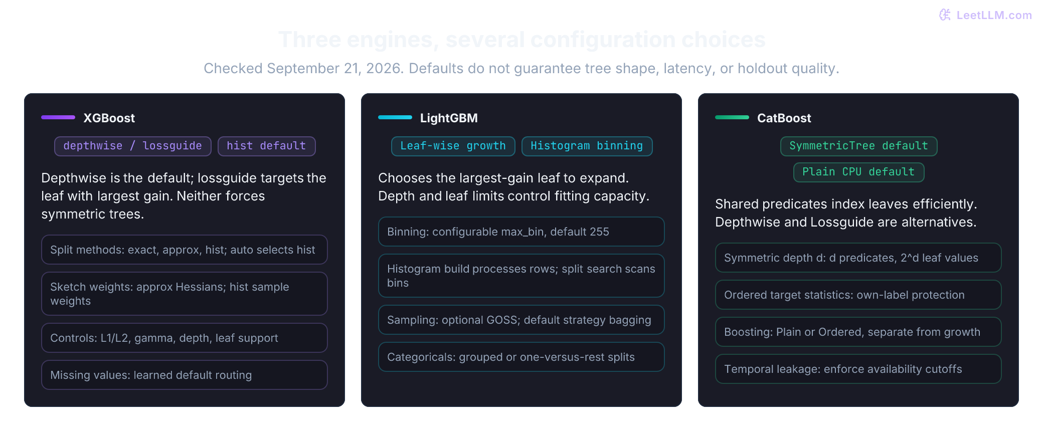
- XGBoost:
grow_policy="depthwise"is the default; supported histogram/approximate methods also offer"lossguide". Depth-wise expansion isn't depth-first traversal and doesn't force every branch to the same depth. Split methods includeexact,approx, andhist; currentautoselectshist. Approx uses Hessian-weighted sketches per tree; hist builds a global sketch using supplied sample weights. Column subsampling is configurable, with method-dependent support.[10][11] - LightGBM: Leaf-wise growth chooses the leaf with largest gain;
num_leaves,max_depth, and leaf-support settings control capacity without guaranteeing generalization. Histogram construction still processes rows, roughly for dense rows and features; scanning split bins and subtracting histograms use roughly for bins.max_bindefaults to 255 and is configurable; memory savings depend on the data and representation.[12][13] GOSS is optional:data_sample_strategydefaults tobagging. GOSS retains large-gradient rows and reweights a sampled small-gradient subset; EFB bundles sparse features with little overlap.[14][13] Categorical search can group categories, while small-cardinality features use one-versus-rest splits undermax_cat_to_onehot; declaring a column categorical still matters.[15][13] - CatBoost:
SymmetricTreeis the default growth policy;DepthwiseandLossguidealso exist. A full symmetric depth- tree uses predicates to index leaves, enabling efficient evaluation without a guarantee of zero branch misses. Ordered target statistics address own-label leakage in categorical encoding; Ordered boosting addresses the paper's prediction-shift mechanism. They aren't universal cures for temporal leakage.boosting_typeis a separate choice, and its CPU default isPlain.[16][17]
When a policy needs a score of 0.20 to mean roughly a 20% miss rate, inspect calibration with a reliability curve. Brier score measures overall probability error, not calibration alone. Calibration methods such as isotonic regression or sigmoid fitting need data separate from the base model's fitting rows; their selection must also stay outside May.[18] We don't add calibration in this lab: we select a threshold empirically rather than assume the scores are exact probabilities.
Fit a booster with an explicit stopping rule
This lab uses scikit-learn's GradientBoostingClassifier so the code stays small. It builds an additive model stage by stage and fits each tree to the negative gradient of log_loss. A larger job might use XGBoost, but the stopping question stays the same: which round still helps April?
Fix tree depth and learning rate first. Then train a generous maximum of rounds on January through March. The maximum is a ceiling, not a promise to ship every tree.
Don't use sklearn's validation_fraction helper for this split. When early stopping is enabled with n_iter_no_change, it reserves a stratified random portion of the training matrix, not a later month.[8] April is our later calendar group, so score it yourself with staged_predict_proba and keep that boundary intact.
The first snippet only establishes the 160-round ceiling. The next one compares every stage on January-March and April, so you can see when fit on old rows stops helping future-like rows.
round_search = GradientBoostingClassifier(
    loss="log_loss",
    n_estimators=160,
    learning_rate=0.05,
    max_depth=2,
    random_state=11,
)
round_search.fit(train["X"], train["y"])
print("trained stage cap:", round_search.n_estimators_)trained stage cap: 160train_losses = [
log_loss(train["y"], probabilities[:, 1], labels=[0, 1])
for probabilities in round_search.staged_predict_proba(train["X"])
]
validation_losses = [
log_loss(valid["y"], probabilities[:, 1], labels=[0, 1])
for probabilities in round_search.staged_predict_proba(valid["X"])
]
best_round = int(np.argmin(validation_losses) + 1)
print("round 1 train / april:", round(train_losses[0], 4), round(validation_losses[0], 4))
print("best round:", best_round)
print(f"round {best_round} train / april:", round(train_losses[best_round - 1], 4), round(validation_losses[best_round - 1], 4))
print("round 160 train / april:", round(train_losses[-1], 4), round(validation_losses[-1], 4))round 1 train / april: 0.6163 0.6805
best round: 50
round 50 train / april: 0.3491 0.5643
round 160 train / april: 0.2684 0.5922In this run, training loss falls through round 160, while April's minimum is at round 50. Later losses fluctuate above that minimum. Extra trees improve fitting loss without improving this validation metric, a symptom of overfitting. Another sample or deployment regime could select a different round count.
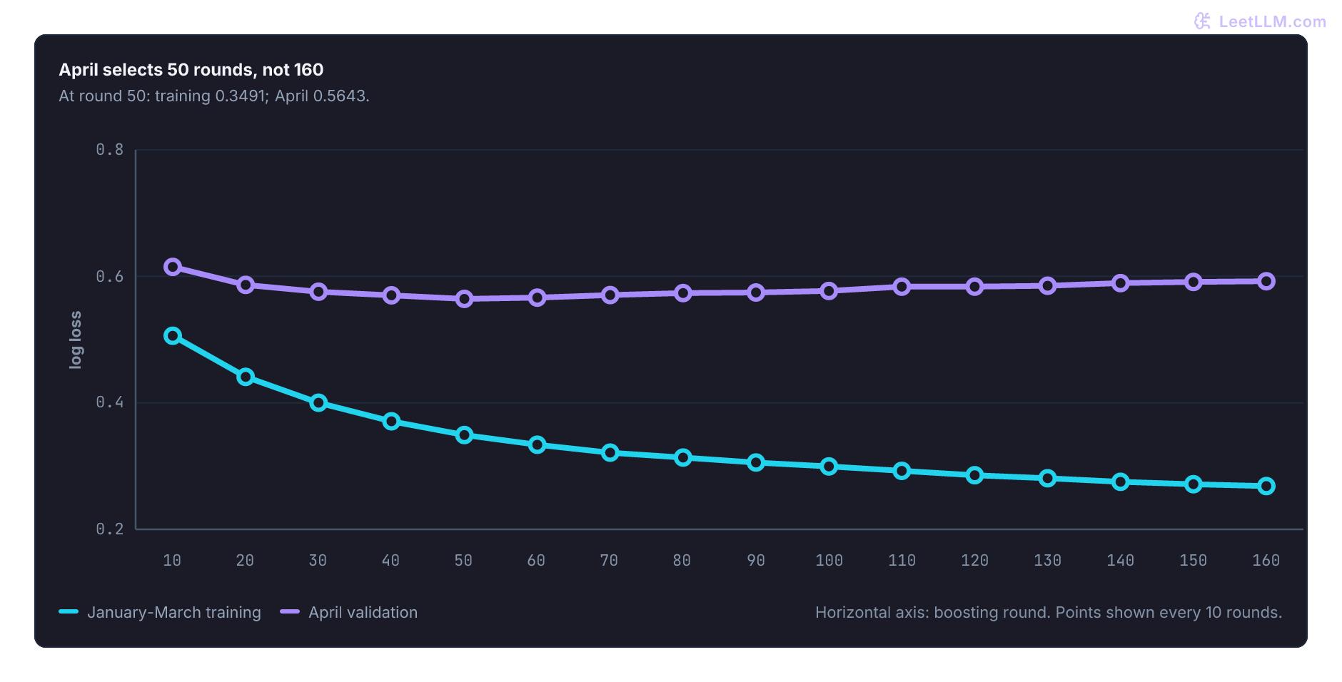
50, training loss drops from 0.3491 to 0.2684 while April loss rises from 0.5643 to 0.5922. The validation minimum selects the candidate, not the training cap.This is retrospective stage selection: we trained all 160 rounds, then selected the minimum April loss. It doesn't save training compute as an online patience-based stopping rule would. Record the validation rows, metric, tie rule, and selected count. argmin takes the first minimum, favoring fewer rounds in a tie. We refit with that count on the same January-March rows; adding April to fitting would change the model and invalidate the threshold selected from these April scores.
candidate = GradientBoostingClassifier(
    loss="log_loss",
    n_estimators=best_round,
    learning_rate=0.05,
    max_depth=2,
    random_state=11,
)
candidate.fit(train["X"], train["y"])
valid_scores = candidate.predict_proba(valid["X"])[:, 1]

print("frozen rounds:", candidate.n_estimators_)
print("rule validation auc:", round(roc_auc_score(valid["y"], rule_valid), 3))
print("boosted validation auc:", round(roc_auc_score(valid["y"], valid_scores), 3))frozen rounds: 50
rule validation auc: 0.731
boosted validation auc: 0.792The booster has April AUC 0.792, versus 0.731 for the binary heartbeat rule. Area under the receiver operating characteristic curve (AUC) measures how often a positive case outranks a negative one, giving half credit to ties. The binary rule creates many ties, so this comparison doesn't measure the full ranking information in heartbeat age itself. More importantly, neither AUC chooses where an operator should intervene.
Validation loss is lowest at round 50 and rises through round 160. Which round count should the frozen candidate use?
Answer
Use round 50, selected on the declared validation slice. Continuing to the training cap would keep trees that improved training fit but worsened held-out loss.
Measure threshold cost, not AUC alone
The classifier outputs a score, not an action. The scheduler still has to choose whether to intervene, notify, or leave a job on its normal path. A missed priority SLA can cost more than an unnecessary notification, so 0.50 is not a neutral operating policy.
Search candidate thresholds on April only. Start with a coarse grid to expose a mistake: if its best threshold is the lowest one tested, values below it may be better. Then evaluate every distinct validation score, plus all-alert and no-alert boundaries. Predictions use score >= threshold, so these candidates represent every distinct single-threshold decision set on April. The sort key minimizes cost and breaks ties toward the lower threshold.
thresholds = [0.15, 0.20, 0.25, 0.30, 0.40]
for threshold in thresholds:
    stats = cost_stats(valid, valid_scores, threshold)
    print(
        f"threshold={threshold:.2f} cost={stats['cost']} "
        f"priority_misses={stats['priority_misses']}"
    )

complete_thresholds = np.r_[0.0, np.unique(valid_scores), np.nextafter(1.0, 2.0)]
selected_threshold = float(min(
    complete_thresholds,
    key=lambda threshold: (cost_stats(valid, valid_scores, threshold)["cost"], threshold),
))
april_rule = cost_stats(valid, rule_valid.astype(float), threshold=0.50)
april_boosted = cost_stats(valid, valid_scores, selected_threshold)
print("selected threshold:", round(selected_threshold, 6))
print("april rule cost:", april_rule["cost"])
print("april always-alert cost:", always_alert_valid["cost"])
print("april boosted cost:", april_boosted["cost"])
assert april_boosted["cost"] <= always_alert_valid["cost"]threshold=0.15 cost=1316 priority_misses=6
threshold=0.20 cost=1884 priority_misses=10
threshold=0.25 cost=1912 priority_misses=10
threshold=0.30 cost=2038 priority_misses=11
threshold=0.40 cost=2604 priority_misses=14
selected threshold: 0.062667
april rule cost: 1560
april always-alert cost: 656
april boosted cost: 568The coarse grid picks 0.15 at cost 1316, losing to always alerting at 656. Complete search selects approximately 0.062667 at cost 568: it catches all 58 misses and suppresses 11 false alarms. Keep the full-precision threshold; the rounded number is for display.
This is the minimum observed April cost within the single global threshold family. It isn't a confirmation of the priority-tier Bayes threshold: the model scores weren't calibrated, the policy family differs, and April is finite. Both rounds and threshold were selected on April, so its reported improvement includes selection optimism. May supplies later evidence.
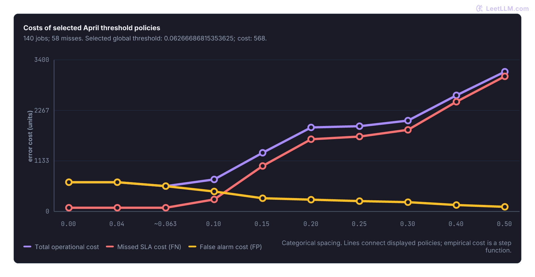
568; 0.50 costs 3134. These are empirical fixture results, not a smooth Bayes-risk curve or a guarantee about later jobs.Freeze the round count, threshold, and cost policy together. May can be opened once for final candidate evidence.
test_scores = candidate.predict_proba(test["X"])[:, 1]
test_stats = cost_stats(test, test_scores, selected_threshold)
rule_test = (test["X"][:, heartbeat_age_index] >= 18).astype(int)
may_rule = cost_stats(test, rule_test.astype(float), threshold=0.50)

print("test auc:", round(roc_auc_score(test["y"], test_scores), 3))
print("may rule cost:", may_rule["cost"])
may_always_alert = cost_stats(test, np.ones(len(test["y"])), threshold=0.50)
print("may always-alert cost:", may_always_alert["cost"])
print("test policy:", test_stats)test auc: 0.882
may rule cost: 1044
may always-alert cost: 680
test policy: {'threshold': 0.06266686815353625, 'cost': 584, 'priority_misses': 0, 'tp': 55, 'fp': 73, 'fn': 0, 'tn': 12}May differs through both random sampling and the drift term; one run doesn't isolate their effects. The frozen policy costs 584, below the heartbeat rule's 1044 and always-alert's 680. It catches all 55 misses but alerts on 128 of 140 jobs. Saving 96 synthetic cost units relative to always alerting isn't automatically worth model maintenance. Keep the threshold frozen: May evaluates the earlier choice, not a new search. Now inspect where those results came from.
Gate slices before promotion
Pick required slices before reading test results. An aggregate score can look fine while one workload carries all the misses, so the slice names and thresholds belong in the release contract.
Recall is caught misses divided by all actual misses: for example, catching 9 of 10 gives 0.90. Support matters too. A slice with no positives has undefined recall, and perfect recall on one positive case is weak evidence. Our illustrative gate requires at least 10 SLA-miss jobs per slice, recall of at least 0.90 for priority jobs, and recall of at least 0.85 for large-model jobs. Ten positives is a teaching threshold, not a statistical assurance of future recall. A production gate needs uncertainty and dependency assumptions appropriate to the stakes.
The gate below reports both pieces of evidence. Predict what should happen if a slice has high recall but fewer than 10 positive cases.
def slice_gate(split, scores, threshold, name, mask, minimum_recall, minimum_positives):
    predicted = (scores >= threshold).astype(int)
    stats = confusion(split["y"][mask], predicted[mask])
    positives = stats["tp"] + stats["fn"]
    measured_recall = stats["tp"] / positives if positives else None
    enough_support = positives >= minimum_positives
    passed = enough_support and measured_recall is not None and measured_recall >= minimum_recall
    result = {
        "name": name,
        "rows": int(np.sum(mask)),
        "positives": positives,
        "recall": round(measured_recall, 3) if measured_recall is not None else None,
        "minimum_recall": minimum_recall,
        "minimum_positives": minimum_positives,
        "confusion": stats,
        "passed": passed,
    }
    recall_text = f"{measured_recall:.3f}" if measured_recall is not None else "undefined"
    print(
        f"{name}: positives={positives} recall={recall_text} "
        f"minimum_recall={minimum_recall:.2f} "
        f"minimum_positives={minimum_positives} pass={passed}"
    )
    return result

priority_index = FEATURES.index("priority")
large_model_index = FEATURES.index("large_model")
required_slice_results = [
    slice_gate(
        test,
        test_scores,
        selected_threshold,
        "priority",
        test["X"][:, priority_index] == 1,
        minimum_recall=0.90,
        minimum_positives=10,
    ),
    slice_gate(
        test,
        test_scores,
        selected_threshold,
        "large_model",
        test["X"][:, large_model_index] == 1,
        minimum_recall=0.85,
        minimum_positives=10,
    ),
]
required_slices_pass = all(result["passed"] for result in required_slice_results)
print("all required slices pass:", required_slices_pass)priority: positives=36 recall=1.000 minimum_recall=0.90 minimum_positives=10 pass=True
large_model: positives=31 recall=1.000 minimum_recall=0.85 minimum_positives=10 pass=True
all required slices pass: TrueBoth required slices pass with recall 1.0. They overlap, so they aren't independent replications, and always alerting would also pass these recall gates. Interpret recall together with the cost and alert-volume comparison. A retrain, feature shift, or threshold edit can break one segment while aggregate metrics still look acceptable.
Exercise the gate's boundaries before relying on it. These masks simulate no positive cases and nine perfectly detected positive cases; neither should pass a ten-positive requirement.
empty = slice_gate(
    test, test_scores, selected_threshold, "empty",
    np.zeros(len(test["y"]), dtype=bool), 0.85, 10,
)
nine_mask = np.zeros(len(test["y"]), dtype=bool)
nine_mask[np.flatnonzero(test["y"] == 1)[:9]] = True
nine = slice_gate(
    test, np.ones(len(test["y"])), selected_threshold, "nine positives",
    nine_mask, 0.85, 10,
)
assert empty["recall"] is None and not empty["passed"]
assert nine["recall"] == 1.0 and not nine["passed"]empty: positives=0 recall=undefined minimum_recall=0.85 minimum_positives=10 pass=False
nine positives: positives=9 recall=1.000 minimum_recall=0.85 minimum_positives=10 pass=FalseTo diagnose a gate, reproduce one predeclared failure: change only the threshold to 0.50 and leave the fitted trees untouched. This is a teaching stress test, not permission to tune on May. A real revision prompted by May needs fresh final evidence.
bad_threshold = 0.50
bad_slice_results = [
    slice_gate(
        test,
        test_scores,
        bad_threshold,
        "priority",
        test["X"][:, priority_index] == 1,
        minimum_recall=0.90,
        minimum_positives=10,
    ),
    slice_gate(
        test,
        test_scores,
        bad_threshold,
        "large_model",
        test["X"][:, large_model_index] == 1,
        minimum_recall=0.85,
        minimum_positives=10,
    ),
]
print("release blocked:", not all(result["passed"] for result in bad_slice_results))priority: positives=36 recall=0.722 minimum_recall=0.90 minimum_positives=10 pass=False
large_model: positives=31 recall=0.645 minimum_recall=0.85 minimum_positives=10 pass=False
release blocked: TrueNothing about the fitted trees changed. The threshold edit alone drops priority recall from 1.0 to 0.722 and large-model recall from 1.0 to 0.645. Versioning only the model file would miss a policy regression.
Why doesn't a higher AUC choose the production intervention threshold?
Answer
AUC measures ordering across thresholds. Operations still needs a threshold chosen against concrete false-alarm and missed-SLA costs, including critical slices such as priority jobs.
Interpret attributions and optimize serving latency
An operator needs to understand which inputs drove an alert and whether scoring meets the application's measured latency budget. Explanation and profiling answer different questions.
Attribution: TreeSHAP vs global split gain
Gain, split count, and impurity decrease are different summaries; check the estimator's definition. They can favor features with many candidate splits and distribute credit unevenly among correlated inputs. None gives the direction of one feature's contribution to one job's score.
TreeSHAP provides local Shapley attributions for a specified explanation game. The original tree algorithm avoids exhaustive coalition enumeration with an procedure, where is tree count, maximum leaves, and maximum depth. Generic exact enumeration can be exponential, but model-agnostic approximations also exist.[19] Exactness depends on the selected game and supported implementation; it doesn't resolve every ambiguity about correlated features.
Record the background and feature_perturbation. Current TreeExplainer uses interventional handling when auto has background data and tree-path-dependent handling otherwise. Those assumptions can change the attribution. Also record model_output: contributions to a raw logit aren't probability percentage points.[20]
For the explained output :
Here is the base output under the chosen background convention. Each averages the feature's marginal contribution across coalitions under that convention.[20]
Check the units with a hypothetical raw-score explanation: a base logit of -1.00 plus contributions +0.42 and +0.26 gives -0.32, or probability about 0.421. Adding those numbers directly to a probability would be wrong. This arithmetic is illustrative, not a computed explanation of our candidate.
Use local attributions to choose an investigation. A large contribution from ticket_escalated_flag suggests inspecting its lineage and availability clock; it doesn't prove the column leaked. Correlated inputs and genuine predecision escalations can also explain reliance. A waterfall plot explains model output, not whether the inputs are trustworthy or changing a feature would improve the job's outcome. An alert payload should include the actual values, attributed output units, feature version, and freshness.
Serving latency: count work, then measure the request
The selected candidate has fewer trees than the search cap. That is verifiable; a fixed speedup or sub-millisecond p99 isn't. Latency depends on the runtime, hardware, tree layout, batch size, threads, feature retrieval, validation, and concurrent load.
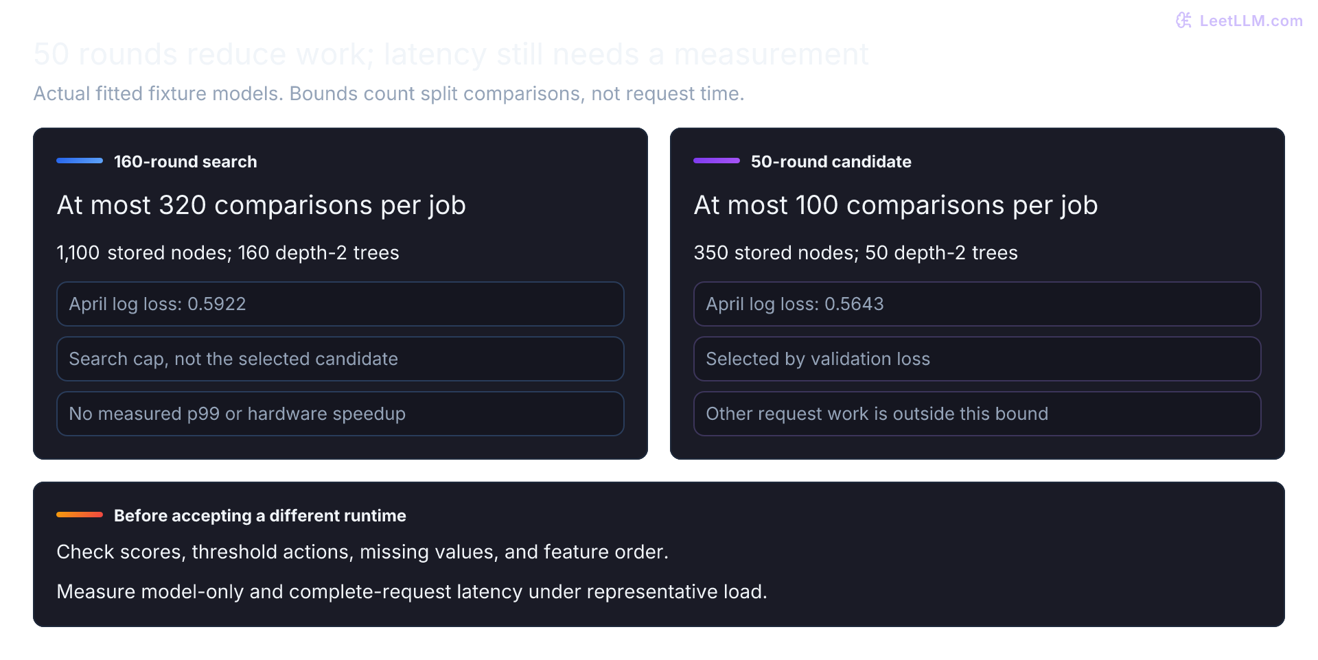
A Python API doesn't imply per-node interpreted traversal. Scikit-learn's tree implementation already stores node arrays and traverses them in compiled code. Irregular accesses and data-dependent branches can still matter, but a profile must establish their cost on the actual workload.[21] Neither 64-byte alignment nor zero branch misses is a universal runtime contract.
As checked September 21, 2026, Treelite is a model exchange/serialization library; its compiler moved to TL2cgen. TL2cgen generates C code and native binaries from supported Treelite models.[22][23] ONNX is another possible serving representation when conversion supports the estimator. None guarantees a speedup.
Treat truncation, pruning, or a new runtime as candidate changes. Removing trees can change probabilities and threshold actions even when individual weights look small. Check validation quality and critical slices, then compare scores and actions near the full-precision threshold, missing-value handling, and feature order. Measure latency under representative load, separating model-only timing from the complete request.
for name, fitted_model in [("search", round_search), ("selected", candidate)]:
    fitted_trees = fitted_model.estimators_.ravel()
    comparison_bound = sum(tree.tree_.max_depth for tree in fitted_trees)
    stored_nodes = sum(tree.tree_.node_count for tree in fitted_trees)
    print(
        f"{name}: trees={len(fitted_trees)} "
        f"comparison_bound={comparison_bound} nodes={stored_nodes}"
)search: trees=160 comparison_bound=320 nodes=1100
selected: trees=50 comparison_bound=100 nodes=350Ship a model that can be operated
The model file is only one part of a releasable candidate. Export the evidence that explains both the score and the action it triggers:
| Artifact | Why it matters |
|---|---|
feature_contract.json | records column meanings, units, availability times, and missing-value rules |
split_manifest.json | records row IDs, grouping, cutoff times, and label-availability checks |
model.skops or model.onnx | versioned fitted model |
threshold_policy.json | turns score into action |
slice_metrics.json | records required-slice support and regressions |
serving_schema.json | defines the names, types, ranges, and shape the server must validate |
Create a compact receipt for the candidate. Choose persistence based on how the serving process uses the model: ONNX suits a score-only runtime that doesn't need the Python object, while skops.io lets you inspect untrusted types before loading the object. Pickle, joblib, and cloudpickle are trusted-source-only because loading them can execute code. None of those Python formats support loading an estimator trained on a different scikit-learn version, so pin Python, scikit-learn, NumPy, SciPy, and the serializer together.[24]
The receipt below records measured results and a narrow evaluation gate: beat both baselines and pass the required slices. It doesn't serialize the estimator or bind its bytes, training data, source revision, or dependency lock. A hash identifies this JSON payload, not the model it describes. Operational checks remain pending even if the metric gate passes.
baseline_costs = {"heartbeat_rule": may_rule["cost"], "always_alert": may_always_alert["cost"]}
beats_baselines = all(test_stats["cost"] < value for value in baseline_costs.values())
evaluation_passed = beats_baselines and required_slices_pass
receipt = {
    "artifact": "sla-risk-candidate-v1",
    "feature_contract": "point-in-time-snapshot-v1",
    "model": {
        "family": "gradient_boosted_trees",
        "learning_rate": 0.05,
        "max_depth": 2,
        "rounds": best_round,
    },
    "policy": {
        "sla_risk_threshold": selected_threshold,
        "costs": {
            "false_alarm": 8,
            "standard_miss": 60,
            "priority_miss": 150,
        },
    },
    "split_manifest": {"train": "Jan-Mar", "validation": "April", "test": "May"},
    "test_auc": round(roc_auc_score(test["y"], test_scores), 3),
    "test_policy": test_stats,
    "baseline_costs": baseline_costs,
    "beats_baselines": beats_baselines,
    "required_slice_metrics": required_slice_results,
    "required_slices_pass": required_slices_pass,
    "evaluation_passed": evaluation_passed,
    "release_status": "operational_checks_pending" if evaluation_passed else "blocked",
}
payload = json.dumps(receipt, sort_keys=True)
print("release status:", receipt["release_status"])
print("frozen rounds and threshold:", best_round, selected_threshold)
print("receipt sha256:", sha256(payload.encode()).hexdigest()[:12])release status: operational_checks_pending
frozen rounds and threshold: 50 0.06266686815353625
receipt sha256: f0088a0e1691Before promotion, attach the actual model digest, immutable data/split identifiers, code revision, dependency versions, and validation results. Check schema enforcement, realistic serving latency, alert capacity, rollback behavior, and the delayed-label review process. Shadow traffic can expose serving problems without letting candidate scores trigger interventions, but it still consumes resources and needs access controls. It can't establish intervention benefit by itself.
The model saved twelve false alarms in May compared with always alerting. Whether that benefit pays for operating it remains a product decision, not a consequence of passing two recall gates.