Personalize this lesson
Adapt explanations and teaching visuals to your background and preferred voice.
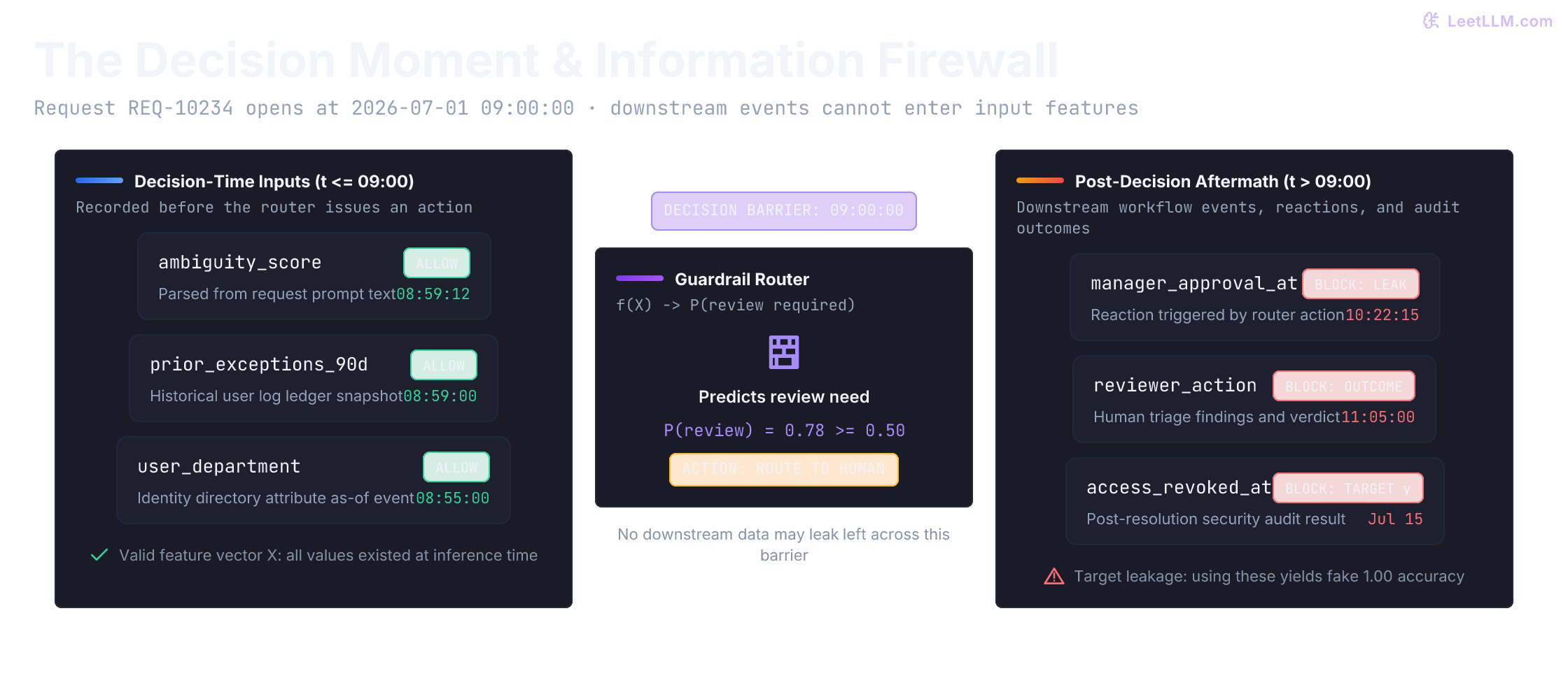
Request REQ-10234 lands on your access gateway at 09:00:00. By 10:22, a manager approves it. Two weeks later, on July 15, a quarterly compliance audit discovers a policy violation and revokes the grant. If you build a model on finished database rows, those later fields look like gold: they predict whether a ticket needed review with near-perfect accuracy. But when the automated router had to make its choice at 09:00:00, none of those downstream events existed yet.
Every machine learning system deployed in production is an engine for making decisions under uncertainty. In empirical risk minimization, our training algorithm optimizes a hypothesis to minimize loss across an available training sample of observations:
Because the model parameters adapt directly to that exact sample, training error is systematically optimistic. The true metric we care about is the out-of-sample risk (or population risk) across the unseen data-generating distribution :
The difference between what our model scores on training data and how it performs in the wild is the generalization gap, .[1]
Offline evaluation exists to estimate this out-of-sample risk honestly before code touches live traffic. Data leakage occurs when information from the target, from future timestamps, or from held-out evaluation entities contaminates the training pipeline. Leakage shrinks the measured generalization gap during development to zero, handing you a mirage: a model that looks flawless on paper but falls apart the second it hits production traffic.
Start at the decision moment
You're building a production guardrail that predicts, the moment a request opens, whether it must route to mandatory human review. The compliance audit supplies the ground-truth label later, applying the security policy in place when the ticket opened. At prediction time, manager approvals, reviewer triage logs, and grant revocation outcomes don't exist yet.
For REQ-10234, the decision timestamp is 2026-07-01 09:00:00.
| Field | When it exists | Valid at opening? | Why |
|---|---|---|---|
ambiguity_score | Before opening | Yes | Extracted from submitted request text |
prior_policy_exceptions_90d | Before opening | Yes | User history already recorded in security logs |
manager_approval_received_at | After evidence request | No | The router's own action can create this event |
access_revoked_after_audit | After resolution | No | Reveals the post-resolution outcome |
needs_review | After audit | Label only | Ground truth target that the guardrail predicts |
Write this feature contract before touching any model code. If a field didn't exist when the action was chosen, it can't enter features, prompt context, retrieval documents, or preprocessing statistics.
Predict the audit before running it: the two 08:59 fields should be allowed, while manager approval and audit revocation must be blocked.
1from datetime import datetime
2
3decision_at = datetime.fromisoformat("2026-07-01T09:00:00")
4fields = [
5    ("ambiguity_score", "2026-07-01T08:59:00"),
6    ("prior_exceptions_90d", "2026-07-01T08:59:00"),
7    ("manager_approval_at", "2026-07-01T10:22:00"),
8    ("access_revoked_at", "2026-07-15T12:00:00"),
9]
10
11for field, observed_at in fields:
12    known = datetime.fromisoformat(observed_at) <= decision_at
13 print(f"{field:22} {'ALLOW' if known else 'BLOCK'}")1ambiguity_score ALLOW
2prior_exceptions_90d ALLOW
3manager_approval_at BLOCK
4access_revoked_at BLOCKThe two blocked fields help downstream forensic analysis, but they aren't valid inputs for the opening decision. Observation time means when the system could actually read the value from its datastores, not merely when the real-world event happened. If an engineer changes their role in HR at 08:50, but the LDAP cache only syncs at midnight, that role update isn't available to an 09:00 decision.
Timestamp audits catch obvious future fields, but derived features need the same scrutiny. Rebuild them from strict as-of snapshots and inspect their aggregation windows. An offline database join can stamp a record at 08:59 while aggregating log rows that arrived at 11:00.
Labels demand an independent audit. A June request audited in August can't train a model deployed on July 1, even though the request itself is weeks old. Training requires both the request features and the ground-truth label to be available prior to the model-fit cutoff. Held-out validation labels can arrive later, because they score predictions frozen at the decision moment.
Why is manager_approval_received_at invalid even though it appears in every completed historical database record?
Answer
The model makes its routing decision before an approval request is ever sent. Using that timestamp gives the model information caused by downstream workflow actions, turning evaluation into an unrealistic simulation where the model sees the consequences of its own decisions.
Train, validation, and test have different jobs
Knowing which columns are available at decision time doesn't complete your evaluation design. To estimate out-of-sample risk honestly, you need three non-negotiable data roles. Confusing their boundaries is the fastest way to mislead your team about a model's true capability.[1]
| Split | Allowed use | Must not do |
|---|---|---|
| Train | Fit model weights, tree splits, tokenizers, scalers, and feature selectors | Claim this score estimates deployment performance |
| Validation | Tune hyperparameters, calibrate probability thresholds, select architectures | Reuse it as an untouched final estimate |
| Test | Estimate out-of-sample risk once after all design decisions are frozen | Inspect errors, tweak features or thresholds, and re-report the score |
To estimate performance on future access requests, use a chronological train, validation, and test split:
- January through June: training.
- July: validation for tuning features and choosing the review threshold.
- August: locked test, opened exactly once after all choices are frozen.
The small fixture below isolates month assignment. It uses two requests per month: 12 training requests, 2 validation requests, and 2 locked test requests. These small counts demonstrate the partitioning logic, not a production-scale evaluation sample.
1episodes = [
2    {"request": f"{month}-{index}", "month": month}
3    for month in range(1, 9)
4    for index in range(2)
5]
6
7train = [row for row in episodes if row["month"] <= 6]
8validation = [row for row in episodes if row["month"] == 7]
9test = [row for row in episodes if row["month"] == 8]
10
11assert len(train) == 12
12assert len(validation) == 2
13assert len(test) == 2
14print("train requests =", len(train), "months = 1..6")
15print("valid requests =", len(validation), "months = 7")
16print("test requests =", len(test), "months = 8 (locked)")1train requests = 12 months = 1..6
2valid requests = 2 months = 7
3test requests = 2 months = 8 (locked)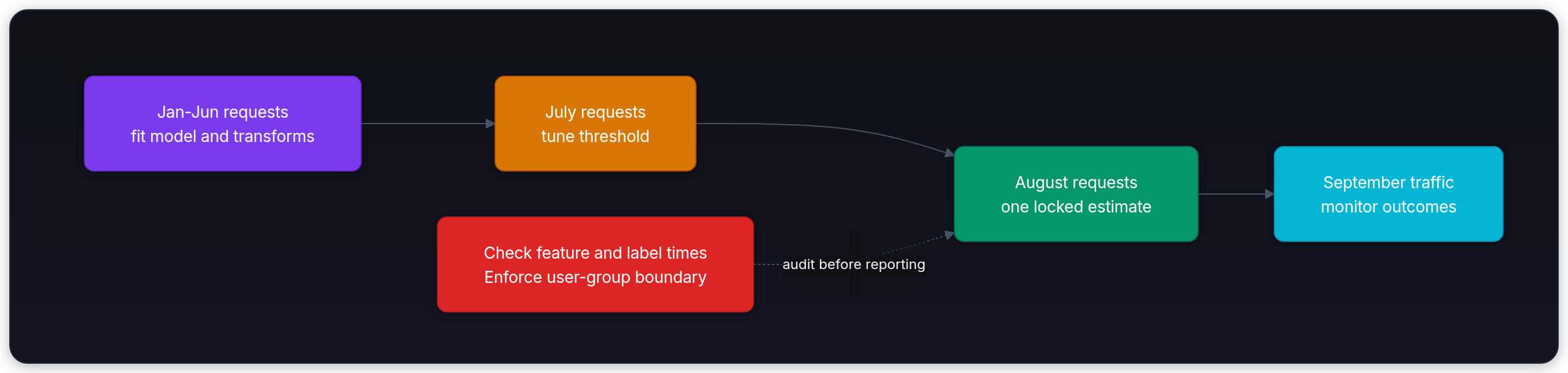
January through June fits parameters, July selects thresholds, and August estimates frozen performance. July's ground-truth labels must be available before the August system is locked; otherwise, move the test window later.
The most common real-world failure mode here is test-set hill-climbing. An engineer evaluates candidate model A on August data, gets a disappointing result, tweaks a few features, adjusts the classification threshold, and re-evaluates candidate model B on the same August data. If model B scores higher, they declare victory and ship it.
That reported score is invalid. The moment August error feedback guides a development choice, August stops being an untouched out-of-sample holdout; it becomes an informal validation set. Its score absorbs selection bias, making the system look more accurate than it actually is.[1] If test results force an architecture revision, August joins the historical development corpus, and an untouched September window must serve as the new locked test.
Cross-validation rotates the validation job
A single validation month can be unusually forgiving or unusually harsh. Cross-validation (CV) repeats fitting and evaluation across several systematic partitions of development data, reducing the variance of our performance estimate without opening the locked final test.[2]
In standard -fold cross-validation, we partition development data into disjoint subsets (folds) of equal size, . For each iteration , we hold out fold as the validation partition and fit the pipeline on the remaining folds, denoted . The overall cross-validation risk estimate is the average validation loss across all folds:
Choosing involves a classic bias-variance trade-off:
- or : Each fold trains on 80% to 90% of development data. This creates a slightly pessimistic bias (since training on fewer examples slightly understates what the full development set can achieve), but the variance of the estimator remains low.
- Leave-One-Out (LOO, ): Each model fits on samples. Bias is practically zero, but computational cost is severe and variance can be surprisingly high: the fitted models are nearly identical because their training sets overlap by samples, inducing strong positive correlation between fold errors.[1]
When target classes are imbalanced, random -fold splitting introduces another subtle risk: some folds may randomly receive zero positive examples. In access routing or fraud detection, where policy violations might make up only 2% of traffic, Stratified K-Fold guarantees that every fold preserves the exact class proportions of the overall dataset.
Suppose five earlier-history folds give these F1 scores for our review guardrail: 0.67, 0.75, 0.58, 0.83, and 0.71. F1 combines precision and recall: how many flagged tickets genuinely needed review, and how many violative tickets were caught.
For the first fold, suppose the guardrail catches 4 needed reviews, sends 3 routine requests to review, and misses 1 needed review. That gives 4 true positives, 3 false positives, and 1 false negative:
The harmonic mean severely penalizes either low precision or low recall. It treats false positives and false negatives symmetrically, which rarely matches business reality: missing a critical policy violation is usually far more dangerous than sending an extra ticket to triage. Keep raw confusion counts beside F1 when choosing production operating points.
1import statistics
2
3fold_f1 = [0.67, 0.75, 0.58, 0.83, 0.71]
4mean_f1 = statistics.mean(fold_f1)
5std_f1 = statistics.stdev(fold_f1)
6
7assert round(mean_f1, 2) == 0.71
8assert round(std_f1, 2) == 0.09
9print("fold F1 =", fold_f1)
10print(f"mean F1 = {mean_f1:.2f}")
11print(f"std F1 = {std_f1:.2f}")1fold F1 = [0.67, 0.75, 0.58, 0.83, 0.71]
2mean F1 = 0.71
3std F1 = 0.09The mean of 0.71 summarizes expected development performance. The sample standard deviation, 0.09, measures dispersion across these five folds. It isn't a standard error of the mean or a confidence interval: because the training sets across folds overlap heavily, the individual fold scores are correlated rather than independent.
Never report the best fold (0.83) as your expected production metric. Investigate the worst fold (0.58) to understand which traffic patterns caused the model to stumble. Note also that the mean of fold F1 scores differs mathematically from the pooled F1 score calculated by aggregating all out-of-fold predictions before evaluating: because F1 is a non-linear ratio, those two summaries will not match.
Standard shuffled cross-validation assumes that rows are exchangeable: swapping rows between folds doesn't violate the underlying distribution. When data has entity grouping or temporal dependencies, that assumption breaks down completely. Stratification balances class counts, but it doesn't prevent a user or future record from crossing the split boundary.[2]
Target leakage: when a feature steals the answer key
Suppose access_revoked_after_audit sits in your historical database table. Because an audit happens weeks after a ticket closes, that column virtually mirrors whether human review was required in the first place. Including it in an opening-time classifier yields an astonishing metric and a completely broken production system.
This is target leakage: when an input feature includes information that is a causal descendant or direct proxy of the label you're trying to predict.
In the lab below, eight held-out requests are scored under two configurations. The honest rule uses only opening-time fields: predict review if ambiguity - 0.9 * policy_support > 0. The leaky rule includes the post-close audit field, which in this dataset directly mirrors the label. Predict which score will look impressive before running the comparison.
1rows = [
2    {"ambiguity": 1.4, "policy": 0, "y": 1},
3    {"ambiguity": -0.2, "policy": 1, "y": 0},
4    {"ambiguity": 0.8, "policy": 0, "y": 1},
5    {"ambiguity": 0.1, "policy": 1, "y": 0},
6    {"ambiguity": 1.1, "policy": 0, "y": 1},
7    {"ambiguity": -0.5, "policy": 1, "y": 0},
8    {"ambiguity": 0.3, "policy": 0, "y": 0},
9    {"ambiguity": 0.6, "policy": 1, "y": 1},
10]
11
12def accuracy(pred, y):
13    return sum(a == b for a, b in zip(pred, y)) / len(y)
14
15y = [row["y"] for row in rows]
16honest = [int(row["ambiguity"] - 0.9 * row["policy"] > 0) for row in rows]
17leaked = list(y)
18
19print(f"decision-time accuracy={accuracy(honest, y):.2f} preds={honest}")
20print(f"future-field  accuracy={accuracy(leaked, y):.2f}")
21assert accuracy(honest, y) == 0.75
22assert accuracy(leaked, y) == 1.01decision-time accuracy=0.75 preds=[1, 0, 1, 0, 1, 0, 1, 0]
2future-field accuracy=1.00The last two rows expose the honest rule's real-world misses: at ambiguity=0.3 it predicts review but the label is 0; at ambiguity=0.6 with policy support it predicts no review but the label is 1. Six of eight honest predictions match, giving an authentic 0.75 accuracy.
The leaked field matches every single label because it literally copies the ground truth. When your offline model scores an improbable 1.00 accuracy or 0.999 AUC, it hasn't achieved artificial superintelligence. You've simply handed the model an answer key that won't exist at 09:00:00 on Monday morning.
Clustered entities change the generalization claim
A standard random row split assumes every observation is independently generated. In production software, data points almost always cluster around entities: users, patient IDs, enterprise organizations, or host machines.
If your product promise is "this model generalizes to brand-new users," but each user's earlier requests appear in the training split while later requests appear in validation, your evaluation is answering the wrong question. The model doesn't need to learn generalizable security principles: it can simply memorize user-specific idiosyncrasies, such as habitual request times, specific cloud resource IDs, or writing style.
The fixture below isolates this failure mode. Eight users each submit two identical requests, and the label is a user-specific attribute. The model is a simple lookup table: if a user appeared in training, repeat their known label; otherwise fall back to 0.
The first split puts one row from every user on each side. The second split holds out entire users using a group boundary.
1rows = []
2for user_index in range(8):
3    user_id = f"u{user_index:02d}"
4    label = user_index % 2
5    rows.extend([(user_id, label), (user_id, label)])
6
7def lookup_accuracy(train_idx, val_idx):
8    memory = {rows[i][0]: rows[i][1] for i in train_idx}
9    correct = 0
10    for i in val_idx:
11        user_id, label = rows[i]
12        pred = memory.get(user_id, 0)
13        correct += pred == label
14    return correct / len(val_idx)
15
16row_train = list(range(0, 16, 2))
17row_val = list(range(1, 16, 2))
18group_train = [i for i, (user_id, _) in enumerate(rows) if int(user_id[1:]) < 4]
19group_val = [i for i, (user_id, _) in enumerate(rows) if int(user_id[1:]) >= 4]
20
21row_acc = lookup_accuracy(row_train, row_val)
22group_acc = lookup_accuracy(group_train, group_val)
23assert row_acc == 1.0
24assert group_acc == 0.5
25print(f"paired-row accuracy = {row_acc:.2f}")
26print(f"held-out-user accuracy = {group_acc:.2f}")1paired-row accuracy = 1.00
2held-out-user accuracy = 0.50The 1.00 score measures recognition of users already represented in training. The 0.50 score is the honest unseen-user result for this balanced fixture and its fallback rule.
When you promise generalization across new entities, use GroupKFold so every row belonging to an entity stays strictly on one side of the fold boundary. Simply dropping the explicit user_id column isn't enough: high-capacity models easily reconstruct user identity from correlated behavioral signals.[2]
Why should every row from one user stay in the same fold when testing generalization to new users?
Answer
Rows from the same user share behavioral patterns, vocabulary, and environment fingerprints. Letting that entity span train and validation allows the model to memorize user-specific identities rather than learning transferable patterns that work on new people.
Preprocessing can learn from validation rows
Data leakage doesn't require an explicit future column. A feature scaler, missing-value imputer, target encoder, principal component analysis (PCA) projection, or feature selector learns parameters during its fit step. If you run .fit() or .fit_transform() on your entire dataset before splitting, validation data has already corrupted your pipeline.[3]
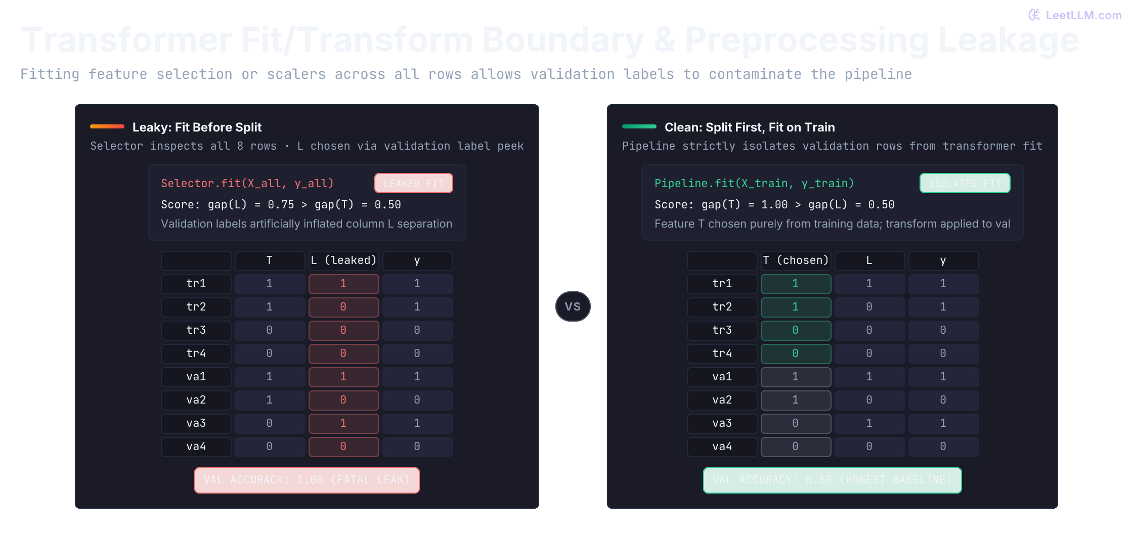
Consider eight rows and two candidate features: T and L. Column T perfectly mirrors training labels and is noisy on validation. Column L is weak on training and copies validation labels.
Our selector picks the column with the larger absolute difference between class means: . On training rows, T achieves while L achieves . But across all eight rows, validation labels join the calculation, inflating L's separation to while dragging T down to .
Both paths fit a nearest-mean classifier on training rows only. Only the feature selector's input changes: all eight rows, or training rows alone. Predict which column each path chooses before running the script.
1T = [1, 1, 0, 0, 1, 1, 0, 0]
2L = [1, 0, 0, 0, 1, 0, 1, 0]
3y = [1, 1, 0, 0, 1, 0, 1, 0]
4train, val = range(4), range(4, 8)
5
6def mean_gap(col, idx):
7    ones = [col[i] for i in idx if y[i] == 1]
8    zeros = [col[i] for i in idx if y[i] == 0]
9    return abs(sum(ones) / len(ones) - sum(zeros) / len(zeros))
10
11def nearest_mean_accuracy(col, train_idx, val_idx):
12    ones = [col[i] for i in train_idx if y[i] == 1]
13    zeros = [col[i] for i in train_idx if y[i] == 0]
14    mean_one = sum(ones) / len(ones)
15    mean_zero = sum(zeros) / len(zeros)
16    correct = 0
17    for i in val_idx:
18        pred = 1 if abs(col[i] - mean_one) < abs(col[i] - mean_zero) else 0
19        correct += pred == y[i]
20    return correct / len(val_idx)
21
22print(f"train gap T={mean_gap(T, train):.2f} L={mean_gap(L, train):.2f}")
23print(f"all   gap T={mean_gap(T, range(8)):.2f} L={mean_gap(L, range(8)):.2f}")
24columns = {"T": T, "L": L}
25leaky_name = max(columns, key=lambda name: mean_gap(columns[name], range(8)))
26safe_name = max(columns, key=lambda name: mean_gap(columns[name], train))
27leaky_acc = nearest_mean_accuracy(columns[leaky_name], train, val)
28safe_acc = nearest_mean_accuracy(columns[safe_name], train, val)
29print(f"select {leaky_name} on all rows val acc={leaky_acc:.2f}")
30print(f"select {safe_name} on train    val acc={safe_acc:.2f}")
31assert (mean_gap(T, train), mean_gap(L, train)) == (1.0, 0.5)
32assert (mean_gap(T, range(8)), mean_gap(L, range(8))) == (0.5, 0.75)
33assert leaky_acc == 1.0
34assert safe_acc == 0.51train gap T=1.00 L=0.50
2all gap T=0.50 L=0.75
3select L on all rows val acc=1.00
4select T on train val acc=0.50On training rows alone, T wins decisively (1.00 vs 0.50). Across all eight rows, L wins (0.75 vs 0.50) because validation labels entered the selection contest. The train-fitted classifier on L then scores 1.00 on those same validation rows. Select on training rows only, and validation accuracy falls to genuine chance (0.50).
In a famous scikit-learn experiment with 10,000 completely random features and random noise labels, selecting the top 100 features before splitting yields 76% validation accuracy on pure white noise! Selecting features strictly inside each training split produces the true 50% chance baseline.[3]
The production cure for preprocessing leakage is architectural: encapsulate every transform inside a Pipeline:
1from sklearn.feature_selection import SelectKBest, f_classif
2from sklearn.linear_model import LogisticRegression
3from sklearn.model_selection import cross_val_score
4from sklearn.pipeline import Pipeline
5
6pipeline = Pipeline([
7    ("selector", SelectKBest(score_func=f_classif, k=1)),
8    ("classifier", LogisticRegression()),
9])
10# cross_val_score fits selector and classifier on training folds only
11scores = cross_val_score(pipeline, X, y, cv=5)
When passed to cross_val_score, the Pipeline ensures that selector.fit() and classifier.fit() execute strictly on the training fold, while transform() and predict() execute out-of-sample on validation rows. A pipeline won't fix a bad time split or repair a leaked database field, but it completely eliminates transform leakage.
Where should a scaler, imputer, or target encoder be fitted during cross-validation?
Answer
Fit it strictly on each fold's training partition, then apply that fitted transform to the fold's validation partition. Fitting once across all rows leaks validation statistics into the model hypothesis space before training even begins.
Temporal validation: walk-forward, purging, and embargo windows
Access routing faces seasonal traffic, policy shifts, infrastructure migrations, and evolving user habits. A model fitted on August can't predict June in any honest simulation of future performance. Rolling-origin evaluation (walk-forward time-series cross-validation) advances the training cutoff chronologically, ensuring that every validation fold evaluates requests that occurred strictly after its training data.[4]
Expanding historical windows mirror production retraining: you retrain periodically on accumulated historical data. In our access routing timeline, we keep development folds strictly within January through June: train on months 1-2 and validate on 3-4; then expand training to months 1-4 and validate on 5-6. July is the dedicated threshold-selection month, while August remains locked.
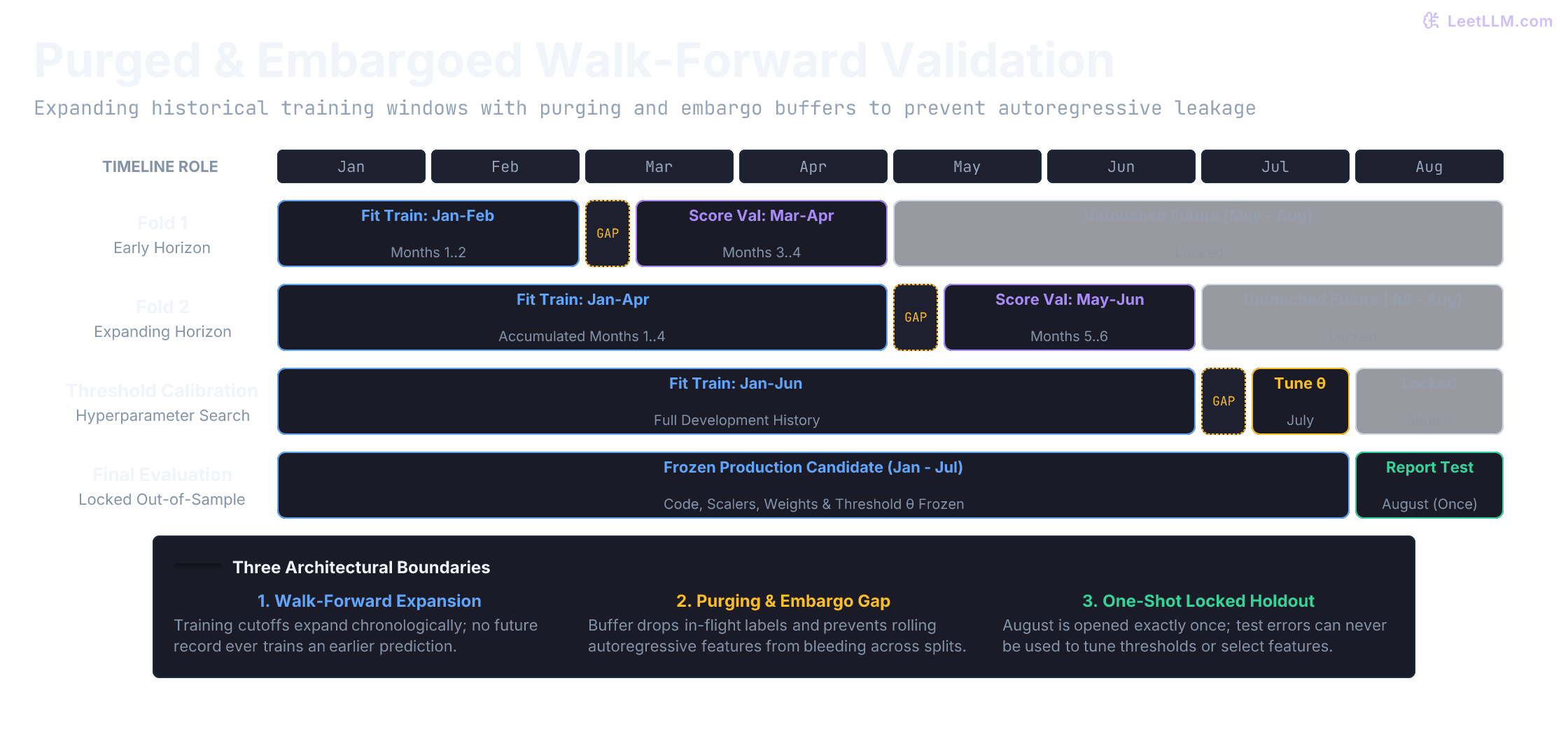
In sequential production systems, chronological ordering alone isn't enough to prevent leakage. Two subtle mechanisms frequently corrupt temporal splits:
- Purging overlapping label horizons: In reality, outcome labels rarely arrive instantaneously. An access ticket opened on June 25 might take 14 days for a security audit to resolve, meaning its label arrives on July 9. If you train on data up to June 30 and validate on July, that late-June training row's label was shaped by events occurring inside the July validation window. Purging removes any training instance whose label resolution horizon extends into the validation window.
- Embargo windows for autoregressive features: Features frequently rely on backward-looking rolling aggregates, such as a user's 7-day request count or 30-day policy exception velocity. On July 1 at 00:05, a request's 7-day velocity is computed from raw events that occurred in late June, which the model already processed during training. Because of autoregression and shared underlying log events, data points immediately following the split boundary are not truly independent. An embargo window places a protective buffer (such as 7 days of unused data) immediately after the training cutoff to eliminate autoregressive feature bleed.
1months = [month for month in range(1, 7) for _ in range(2)]
2folds = [(1, 2, 3, 4), (1, 4, 5, 6)]
3
4for fold, (train_lo, train_hi, val_lo, val_hi) in enumerate(folds, start=1):
5    train = [m for m in months if train_lo <= m <= train_hi]
6    validation = [m for m in months if val_lo <= m <= val_hi]
7    assert max(train) < min(validation)
8    assert max(validation) <= 6  # July selects; August stays locked.
9    print(
10        f"fold {fold}: train <= {max(train)} "
11        f"validate = {min(validation)}..{max(validation)}"
12 )1fold 1: train <= 2 validate = 3..4
2fold 2: train <= 4 validate = 5..6Each fold keeps validation chronologically after training. Refit the complete pipeline, including all encoders and scalers, independently from scratch inside each fold.
Time and group boundaries combined
A future validation month contains both returning and genuinely new users. If your business cares about both, evaluate and report them as distinct slices.
Repeated users aren't automatically leakage: prior user history is legitimate context for a returning-user prediction if that history existed before the decision moment. But a claim about performance on new users requires both a temporal boundary and a group boundary: no user in that validation slice can have prior history in training.
The fixture below freezes training at July 1. Request r2 opened in June, but its label arrives in August, so it can't enter July training. July traffic contains returning user u1 and new user u4.
1from datetime import datetime
2
3# request, user, opening time, time its label becomes available
4rows = [
5    ("r1", "u1", "2026-01-03", "2026-01-10"),
6    ("r2", "u2", "2026-06-20", "2026-08-02"),
7    ("r3", "u3", "2026-06-10", "2026-06-20"),
8    ("r4", "u1", "2026-07-03", "2026-07-10"),
9    ("r5", "u4", "2026-07-05", "2026-07-20"),
10]
11rows = [(r, u, datetime.fromisoformat(t), datetime.fromisoformat(l))
12        for r, u, t, l in rows]
13fit_at = datetime(2026, 7, 1)
14end_at = datetime(2026, 8, 1)
15history = [row for row in rows if row[2] < fit_at]
16train = [row for row in history if row[3] <= fit_at]
17seen_users = {row[1] for row in history}
18july = [row for row in rows if fit_at <= row[2] < end_at]
19new_users = [row for row in july if row[1] not in seen_users]
20returning_users = [row for row in july if row[1] in seen_users]
21
22assert {row[1] for row in train}.isdisjoint(row[1] for row in new_users)
23print("training requests:", [row[0] for row in train])
24print("returning-user July requests:", [row[0] for row in returning_users])
25print("new-user July requests:", [row[0] for row in new_users])1training requests: ['r1', 'r3']
2returning-user July requests: ['r4']
3new-user July requests: ['r5']User u2 is marked as previously seen even though its label isn't ready for training. Newness depends on past activity, not on whether an earlier ticket made it into the training split.
Nested selection and validation overuse
Validation data lets you choose features, tune regularizers, and calibrate decision thresholds. But unlimited search comes with a hidden cost: if you evaluate 5,000 hyperparameter combinations against the same validation split, pure sample noise will eventually win the contest.
Reporting that winning validation score as your expected production performance is another class of leakage: selection bias from validation overuse. Nested cross-validation prevents this by separating model selection from model evaluation:[1]
- Outer loop: Partitions data into outer folds (or walk-forward temporal blocks) that never participate in tuning or model selection.
- Inner loop: For each outer fold, searches hyperparameters, features, and thresholds using internal cross-validation on the remaining development folds only.
- Outer evaluation: Fits the winning inner configuration on the development partition and scores it once on the untouched outer fold.
The average score across the outer folds estimates the generalized error of your entire modeling procedure, not of a specific parameter set chosen after inspecting outer results. If computing nested CV across large models is too expensive, preserve at least one locked, untouched temporal window at the end of your timeline. Treat heavy validation searches as exploratory, never as published claims.
Threshold calibration: validation chooses, test reports
A probabilistic classifier doesn't output binary decisions; it outputs a score or calibrated probability . To act in production, you must set an operating threshold such that when .
Choosing this threshold from your test set is target leakage: test labels directly shape the decision boundary.
In the lab below, July validation data evaluates three candidate thresholds: , , and . Only after selection is locked does August report one final test score. F1 for threshold uses predictions . Predict which threshold July selects before opening August.
1thresholds = [0.30, 0.50, 0.70]
2validation_probability = [0.82, 0.62, 0.58, 0.42, 0.31, 0.12]
3validation_label = [1, 1, 1, 0, 0, 0]
4test_probability = [0.77, 0.49, 0.39, 0.52, 0.66, 0.14]
5test_label = [1, 1, 0, 0, 1, 0]
6
7def f1_score(y, pred):
8    tp = sum(a == 1 and b == 1 for a, b in zip(y, pred))
9    fp = sum(a == 0 and b == 1 for a, b in zip(y, pred))
10    fn = sum(a == 1 and b == 0 for a, b in zip(y, pred))
11    precision = tp / (tp + fp) if tp + fp else 0.0
12    recall = tp / (tp + fn) if tp + fn else 0.0
13    return 0.0 if precision + recall == 0 else 2 * precision * recall / (precision + recall)
14
15validation_f1 = {
16    threshold: f1_score(
17        validation_label, [int(p >= threshold) for p in validation_probability]
18    )
19    for threshold in thresholds
20}
21chosen = max(validation_f1, key=validation_f1.get)
22test_f1 = f1_score(test_label, [int(p >= chosen) for p in test_probability])
23
24for threshold, score in validation_f1.items():
25    print(f"threshold={threshold:.2f} valid_f1={score:.2f}")
26print(f"chosen threshold={chosen:.2f} test_f1={test_f1:.2f}")
27assert validation_f1[0.50] == 1.0
28assert round(test_f1, 2) == 0.671threshold=0.30 valid_f1=0.75
2threshold=0.50 valid_f1=1.00
3threshold=0.70 valid_f1=0.50
4chosen threshold=0.50 test_f1=0.67Threshold 0.50 classifies all six July validation requests perfectly, scoring 1.00. Applying that frozen threshold to August yields two true positives, one false positive, and one false negative, producing an F1 of 4 / (4 + 1 + 1) = 0.67.
Six test rows are far too small for statistical certainty, but the drop illustrates an essential truth: your validation metric was an optimized search score; the locked test metric is your honest out-of-sample estimate. If you had reported July's 1.00 to stakeholders, you would have promised a mirage. If you tweak the threshold after seeing August's errors, you destroy the test set's integrity. Log the chosen threshold, feature contract, and locked test score together.
Modern relevance: benchmark contamination in large language models
The fundamental laws of data leakage don't disappear when tabular rows become prompt tokens, retrieval documents, or public evaluation benchmarks. Large language models (LLMs) face identical boundary failures across every layer of their architecture:
| System | Leakage path | Honest boundary |
|---|---|---|
| Retrieval-augmented generation (RAG) | Chunks from one source document span both tuning sets and evaluation queries | Assign whole source documents before chunking |
| Fine-tuning & instruction tuning | Evaluation questions, worked traces, or ground-truth answers enter SFT corpora | Enforce dataset provenance and hash-based quarantine |
| Public benchmark evaluation | Benchmark test problems (MMLU, GSM8K, HumanEval) exist in pretraining web scrapes | Decontaminate pretraining corpora via n-gram filtering and test on fresh dynamic benchmarks |
For an enterprise access-policy assistant, determine exactly what you're evaluating. If your claim is generalization to new policy manuals, keep each document and its derived queries together. If your claim is answering new questions about an existing, static knowledge base, retrieving from shared documents is intended production behavior, not leakage. Leaking occurs when evaluation queries or reference answers contaminate prompt tuning or embedding models.
The fixture below verifies document-level isolation. Alternating chunks shares every source document across train and test, whereas partitioning complete source pages first shares zero documents.
1documents = {
2    "policy_access": [
3        "temporary admin roles need review",
4        "manager approval may support access grant",
5    ],
6    "policy_incidents": [
7        "sev2 incidents need incident commander approval",
8        "service-owner approval precedes production access",
9    ],
10    "policy_admins": [
11        "privileged role appeal needs audit",
12        "audit stores decision reason",
13    ],
14}
15chunks = [(document, chunk) for document, texts in documents.items() for chunk in texts]
16
17bad_train = chunks[::2]
18bad_test = chunks[1::2]
19bad_overlap = sorted(
20    {document for document, _ in bad_train} & {document for document, _ in bad_test}
21)
22
23safe_train_documents = {"policy_access", "policy_incidents"}
24safe_test_documents = {"policy_admins"}
25safe_train = [(doc, text) for doc, texts in documents.items()
26              if doc in safe_train_documents for text in texts]
27safe_test = [(doc, text) for doc, texts in documents.items()
28             if doc in safe_test_documents for text in texts]
29safe_overlap = sorted({doc for doc, _ in safe_train} & {doc for doc, _ in safe_test})
30
31print("split chunks first shared documents =", bad_overlap)
32print("split documents first shared documents =", safe_overlap)
33assert bad_overlap == ["policy_access", "policy_admins", "policy_incidents"]
34assert safe_overlap == []1split chunks first shared documents = ['policy_access', 'policy_admins', 'policy_incidents']
2split documents first shared documents = []At foundation scale, pretraining corpora swallow trillions of tokens from Common Crawl, GitHub, and books. Those web scrapes frequently contain the exact test splits of standard benchmarks: MMLU, HumanEval, GSM8K, and MATH. A model that achieves 90% on coding benchmarks may simply be recalling memorized repository files rather than demonstrating generalizable program synthesis.
Teams detect and mitigate benchmark contamination using three complementary strategies:
- Exact N-gram overlap filtering: An n-gram is a sequence of consecutive tokens or words. GPT-3 analyzed contamination by checking word overlaps up to 13 words between training data and benchmark tasks.[5] Meta's Llama 3 technical report used 8-gram overlap filtering, discovering that 85% of HellaSwag was contaminated in the pretraining mix, which artificially inflated the 8B model's score by an estimated 14.8 points.[6]
- MinHash and Locality-Sensitive Hashing (LSH): Exact n-grams miss minor rewording. MinHash algorithms find near-duplicate documents and paraphrased questions efficiently across multi-terabyte datasets.
- Perplexity and loss anomaly auditing: If an LLM exhibits an abrupt drop in cross-entropy loss (or perplexity) on benchmark items compared to structurally similar held-out text, it has likely memorized that exact sequence during pretraining.
To stay ahead of web-scrape contamination, modern benchmarks like LiveBench[7] and LiveCodeBench[8] continuously harvest new contest problems and news sources published strictly after model release dates.
The local smoke test below searches for exact 5-gram overlap between training and evaluation prompts:
1training_prompts = [
2    "route privileged access request with required review to human queue",
3    "approve access grant after clear manager approval arrives",
4]
5evaluation_prompts = [
6    "route privileged access request with required review to human queue",
7    "send an ambiguous admin request to a reviewer",
8]
9
10def ngrams(text, size=5):
11    words = text.lower().split()
12    return {
13        " ".join(words[start : start + size])
14        for start in range(len(words) - size + 1)
15    }
16
17training_grams = set().union(*(ngrams(prompt) for prompt in training_prompts))
18for prompt in evaluation_prompts:
19    overlaps = ngrams(prompt) & training_grams
20    status = "FLAG" if overlaps else "NO EXACT MATCH"
21 print(f"{status}: {prompt}")1FLAG: route privileged access request with required review to human queue
2NO EXACT MATCH: send an ambiguous admin request to a reviewerExact matching flags verbatim copy-paste. It can't catch paraphrases, translations, reworded questions, or syntactically altered code. Conversely, boilerplate phrases like "please review the attached log" can trigger false positives. Use n-gram filters as an initial sieve, paired with semantic embeddings and provenance tracking.
Historical logs don't reveal unchosen actions
Our labs evaluate a supervised guardrail: given request context available at opening, predict whether compliance review was required. That setup doesn't estimate the business return of a brand-new sequential decision policy.
Historical server logs tell you what happened under the action the legacy router took. They can't tell you what would have happened if the router took a different action for that same request. Those missing results are counterfactual outcomes.
In reinforcement learning, off-policy evaluation (OPE) estimates the value of a new policy using logs generated by a historical policy. OPE requires strong assumptions beyond temporal splitting, most notably common support (action coverage): the historical policy must have chosen the new policy's actions with non-zero probability in similar contexts. Logging action propensities (the probability with which the logging policy chose each option) is essential, but it can't recover outcomes for actions that were never explored.[9]
A simulated environment can supply synthetic counterfactual outcomes, but the simulator itself requires validation. To measure true policy impact, pair offline supervised audits with staged canary deployments and randomized online experiments.
Write the production evaluation contract
Before publishing any benchmark or shipping an access guardrail, document your boundaries in a concrete contract:
1Decision moment: request opening, before evidence request or reviewer action
2Allowed features: ambiguity_score, policy_support, prior_policy_exceptions_90d
3Forbidden features: manager_approval_received_at, reviewer_action, access_revoked_after_audit
4Train: January-June requests
5Training labels: available by the model-fit cutoff, not merely attached later
6Validation: July requests; tune thresholds, encoders, and feature selectors here
7Test: August requests; open once after all modeling choices are frozen
8Label timing: July labels must be ready before freezing the August system
9Entity promise: report future returning-user and genuinely new-user slices separately
10Preprocessing: every fit step uses training-fold rows only inside a Pipeline
11Feature snapshot: as-of request opening; aggregation windows terminate before decision time
12Metrics: review-required F1, missed-review count, and false-alarm triage load
A benchmark metric is only as honest as the contract that generated it.
Stress-test the contract
Test your evaluation harness by intentionally breaking one assumption at a time. Predict the failure symptom before comparing it with the analysis below:
- Add
reviewer_actionto the feature availability audit and assign an observation time. Explain why it's label-adjacent target leakage. - Modify
group-leakage-from-repeat-users.pyso the product promise is performance on returning users rather than new users. Does row-wise splitting answer that question, and what time boundary remains critical? - Add a neutral column
N = [0, 1, 1, 0, 0, 1, 1, 0]to the feature selector's dictionary. Calculate its class-mean gaps and predict whether either selected column changes. - Extend the document-chunk lab with a paraphrased evaluation chunk. Why does the exact n-gram matcher miss it, and how would you detect it?
- Write an evaluation contract for the reinforcement learning router. Mark which outcomes are directly observed and which are counterfactual.
What each mutation exposes
reviewer_actionis logged only after human triage begins. It belongs in forensic outcome analysis, never in opening-time feature vectors.- A row-wise split can evaluate returning users if prior history was legitimately available at inference time. You must still enforce a strict temporal boundary so later requests don't leak backward into earlier training instances.
- Feature
Nhas class mean 0.5 for both label classes across all rows. Its separation gap is exactly zero: columnTstill wins honest training selection, and columnLstill wins leaky global selection. - Paraphrases preserve semantic intent while altering exact token sequences. Catch them using MinHash near-duplicate clustering, embedding cosine similarity, or manual audit of high-risk test pairs.
- In an RL contract, historical rewards are observed only for the actions chosen by the production logging policy. Rewards for alternative actions proposed by the new candidate policy are counterfactual and require importance-sampled off-policy estimators.