FlashAttention & Memory Efficiency

Prefix caching reuses KV state across requests that share a prompt prefix. It removes repeated work between requests, not the all-pairs work inside one uncached attention call. FlashAttention attacks the layer below that: it makes each dense attention kernel move far less data through GPU memory.

A coding assistant compares each prompt token with itself and earlier tokens during causal prefill. A simple implementation allocates a full square score matrix, even though the upper triangle is masked. Doubling sequence length quadruples that allocation. At 8,192 tokens, batch 8, and 32 heads, a full matrix of 16-bit scores needs 32 GiB before counting anything else.

FlashAttention computes the same attention operator, but it doesn't park the full score or probability matrix in HBM (High Bandwidth Memory, the large GPU RAM pool).^{[1]Reference 1FlashAttention: Fast and Memory-Efficient Exact Attention with IO-Awareness.https://arxiv.org/abs/2205.14135} When attention IO is the bottleneck, that can raise throughput or let a longer context fit.

The memory wall

Materialized attention first

Make the baseline explicit before looking at the optimization. In the scaled dot-product attention article, each query token scores every key token, normalizes those scores with softmax, and blends the corresponding value vectors.

Suppose you have only three prompt tokens from a failing-test message, and a head dimension of two:

• Query $Q$ is a $3 \times 2$ matrix (one row per token).
• Key $K$ and Value $V$ are also $3 \times 2$.

The scaled score matrix $S = QK^T / \sqrt{2}$ is $3 \times 3$: nine numbers, of which six are valid in causal attention. In general, the scale is $1/\sqrt{d}$ for head dimension $d$. Masking changes which scores contribute, but doesn't shrink a full square allocation.

For $batch=8$, $heads=32$, $seq\_len=8192$ in 16-bit floating point (FP16):

That product is exactly $34{,}359{,}738{,}368$ bytes. This is an illustrative FP16 allocation, not a measurement of PyTorch's math backend: its scaled dot-product attention (SDPA) math implementation keeps intermediates in FP32 for FP16/BF16 inputs, doubling the bytes per score.^{[2]Reference 2torch.nn.functional.scaled_dot_product_attentionhttps://docs.pytorch.org/docs/2.14/generated/torch.nn.functional.scaled_dot_product_attention.html} Probability storage, model weights, other activations, and gradients need separate accounting; whether score and probability buffers coexist depends on the implementation.

Check that prediction with a small calculation before blaming model weights for an out-of-memory error:

batch, heads, sequence, bytes_per_value = 8, 32, 8192, 2
score_bytes = batch * heads * sequence * sequence * bytes_per_value

print(f"score values: {batch * heads * sequence * sequence:,}")
print(f"binary size: {score_bytes / 1024**3:.2f} GiB")
print(f"decimal size: {score_bytes / 1000**3:.2f} GB")

score values: 17,179,869,184
binary size: 32.00 GiB
decimal size: 34.36 GB

GPU memory hierarchy

The score count explains capacity. Now follow those values across the memory hierarchy. A GPU isn't a flat memory space. It has layers:

• On-chip SRAM (static random-access memory) is the tiny, ultra-fast scratchpad right next to the compute cores (registers and shared memory).
• HBM is the large pool of GPU memory (VRAM) that holds model weights and tensors.
• CPU DRAM is host memory outside the GPU, used only when data must leave the card entirely.

Memory hierarchy intuition: On-chip SRAM is a tiny, fast scratchpad beside the compute cores. HBM is much larger, but every revisit costs bandwidth. A materializing attention baseline keeps returning to HBM because the full $n \times n$ score matrix doesn't fit in the scratchpad. FlashAttention keeps only active tiles there at a time.

On an NVIDIA H100, each streaming multiprocessor (SM) has 228 KiB of shared memory and a separate 64K 32-bit register file (256 KiB). A thread block can use at most 227 KiB of shared memory; its actual budget also depends on launch settings and other resident blocks. Shared memory shares physical capacity with the L1 cache.^{[3]Reference 3NVIDIA Hopper Tuning Guidehttps://docs.nvidia.com/cuda/hopper-tuning-guide/index.html} These are local resource limits, not one interchangeable scratchpad spread across the GPU.

Hopper can share memory across SMs within a thread-block cluster, but that doesn't make all SM memory one giant tile buffer. Here, "SRAM" is the paper's simplified fast-memory model. A real kernel separately manages shared memory, registers, and synchronization.

Host RAM bandwidth and bandwidth from host to GPU are different quantities. Neither follows from the GPU's HBM specification. Likewise, local-memory latency depends on the access pattern; don't turn an aggregate SRAM estimate into a fixed latency for every tile.

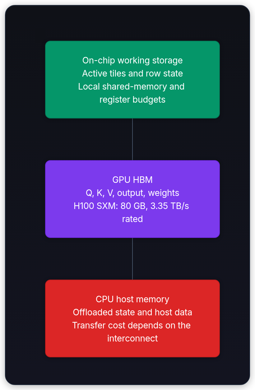
Use this as a capacity pyramid, not a one-way data pipe. Compute wants tiles in SRAM, so ask what happens when the same tile is reused. A materializing baseline keeps bouncing the full $n \times n$ score and probability matrices through HBM, while FlashAttention pays for local bookkeeping to avoid those round-trips.^{[1]Reference 1FlashAttention: Fast and Memory-Efficient Exact Attention with IO-Awareness.https://arxiv.org/abs/2205.14135}

Materialized attention hits the memory bandwidth wall

Follow the physical bytes moved in a materializing baseline. For our running prompt with batch 8, 32 heads, and sequence length 8,192 in FP16:

1. The kernel computes $S = QK^T / \sqrt{d}$ and writes the $32\text{ GiB}$ score matrix $S$ out to HBM.
2. A separate softmax kernel reads all $32\text{ GiB}$ of $S$ back from HBM.
3. The softmax kernel computes probabilities and writes a $32\text{ GiB}$ probability matrix $P$ back to HBM.
4. The value multiply kernel reads all $32\text{ GiB}$ of $P$ and the values $V$ back from HBM to compute $O = PV$.

That adds up to 128 GiB of logical intermediate transfers for this four-pass FP16 baseline, before counting $Q, K, V,$ or the final output $O$. Fusion, datatype, and cache behavior change the physical HBM traffic a profiler observes. FlashAttention avoids those full-matrix intermediates, while still moving inputs, output, and row state.

The roofline model gives a throughput bound from arithmetic intensity $I$: $\min(\text{compute peak},\ I\times\text{bandwidth})$.^{[5]Reference 5Roofline: An Insightful Visual Performance Model for Multicore Architectureshttps://doi.org/10.1145/1498765.1498785} NVIDIA lists 1,979 TFLOPs/s for H100 SXM FP16/BF16 tensor cores with sparsity; halving that advertised figure gives an illustrative dense peak of 989.5 TFLOPs/s.^{[4]Reference 4H100 GPUhttps://www.nvidia.com/en-us/data-center/h100/} Using its 3.35 TB/s bandwidth rating:

$\text{Ridge point} = \frac{989.5 \times 10^{12}\text{ FLOP/s}}{3.35 \times 10^{12}\text{ bytes/s}} \approx 295.4\text{ FLOPs/byte}$

Consider a hypothetical tensor-core workload with intensity 1 FLOP/byte. Its bandwidth roof is only 3.35 TFLOPs/s, about 0.34% of the dense compute peak. That rate ratio is not a measurement of idle cycles. Softmax's reductions and exponentials also use different execution units from tensor-core matrix multiplication, so the tensor-core peak isn't its appropriate compute ceiling.

dense_peak = 1979 / 2  # TFLOPs/s, derived from the sparsity-rated figure
bandwidth = 3.35      # decimal TB/s
intensity = 1.0       # illustrative FLOPs/byte
bandwidth_roof = min(dense_peak, intensity * bandwidth)
print(f"dense compute peak: {dense_peak:.1f} TFLOPs/s")
print(f"ridge point: {dense_peak / bandwidth:.1f} FLOPs/byte")
print(f"illustrative bandwidth roof: {bandwidth_roof:.2f} TFLOPs/s")
print(f"ratio to compute peak: {100 * bandwidth_roof / dense_peak:.2f}%")

dense compute peak: 989.5 TFLOPs/s
ridge point: 295.4 FLOPs/byte
illustrative bandwidth roof: 3.35 TFLOPs/s
ratio to compute peak: 0.34%

Profile memory traffic, execution units, and timing to identify the actual bottleneck. The roofline explains why avoiding transfers can help; it doesn't establish a stall percentage or guarantee that every attention shape is memory-bound.

The FlashAttention algorithm

Core idea: tiling + online softmax

The baseline keeps the attention formula, but its temporary intermediates live too long. FlashAttention combines three ideas instead of materializing the full $n \times n$ attention matrix:

1. Tiles the computation into blocks that fit in SRAM.
2. Uses online softmax to compute exact softmax without seeing all values at once.
3. Never materializes the full attention matrix in HBM.

This block-wise processing strategy avoids quadratic auxiliary score and probability storage. The input, output, and saved row-statistic tensors still scale with sequence length. Before looking at the schedule, predict what should disappear from HBM: temporary score and probability tiles, not the final output.

Trace two data lifetimes in the figure. A materializing baseline writes scores to HBM, reads them for softmax, writes probabilities, and reads those for the value multiply. FlashAttention instead streams tiles through on-chip memory. Besides the output and inputs needed for backward, it saves a row-wise log-sum-exp (LSE) statistic: the log of the sum of exponentiated scores. That statistic lets backward reconstruct probabilities without saving the full matrix.

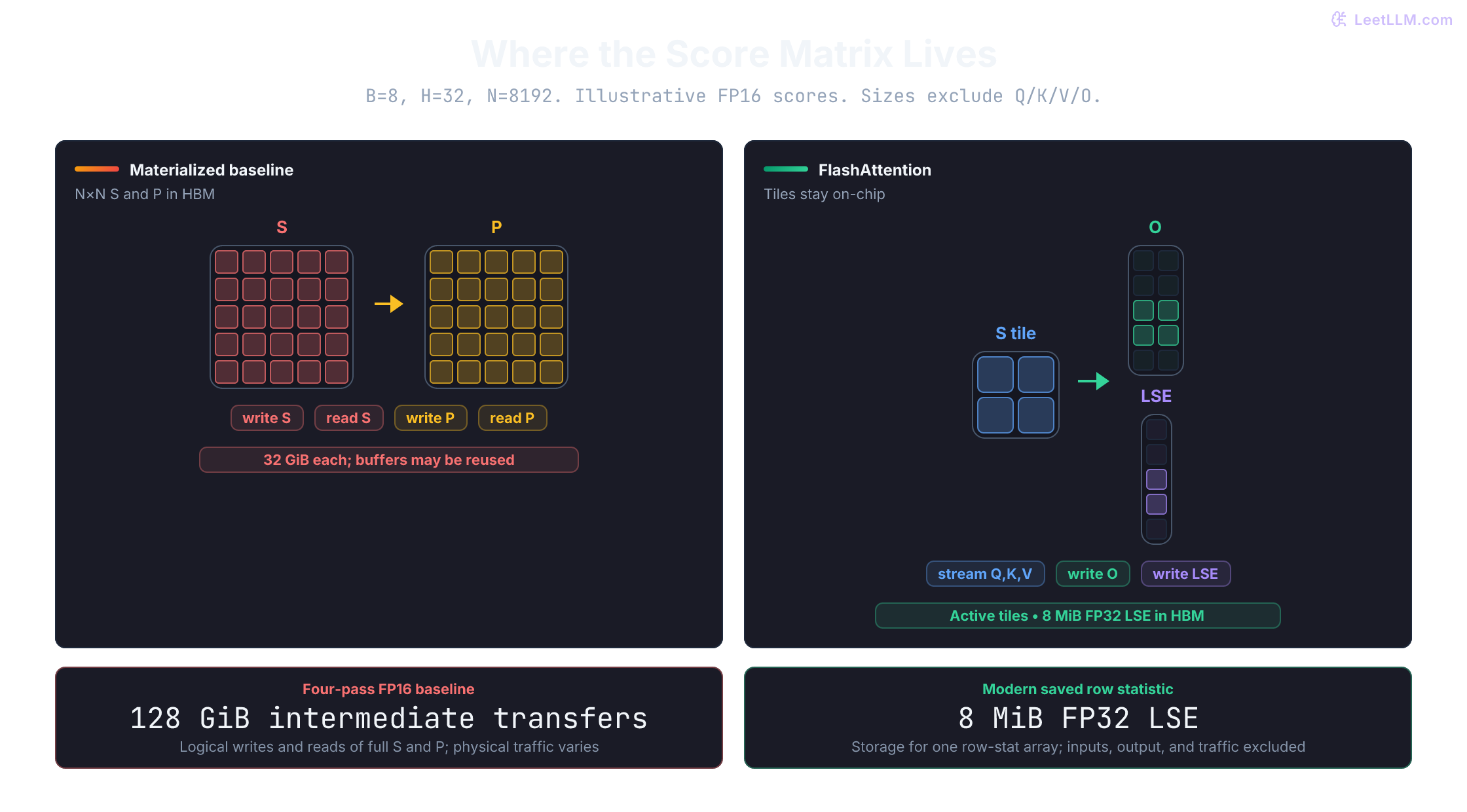
The left path changes memory traffic by revisiting $n \times n$ intermediates in HBM. The right path reuses small blocks in SRAM, then writes the output and compact row statistics. Same operator, different data lifetime.

How tiling fits in SRAM

Tiling changes data lifetime. Pull a block of $Q$, $K$, and $V$ from HBM into SRAM, compute local scores there, and throw the score tile away. During forward execution the kernel writes final output $O$ and, for training, compact row statistics for backward. It doesn't write the full score or probability matrices.

Now the math problem appears. Softmax over a row needs a global max and a global sum. If SRAM holds one K/V tile at a time, you can't see the rest of the row yet. Online softmax is the fix that keeps the result exact.

Ask what must be live at the same time. For 128 query rows, 128 key rows, and head dimension 64, the Q/K/V tiles alone occupy 48 KiB in FP16. Accumulating the output in FP32 adds 32 KiB, and a full FP32 score tile would add 64 KiB. These are logical array sizes, not a shared-memory allocation recipe: kernels distribute state across memory pools, reuse storage, and pipeline loads.

rows, dimension = 128, 64
qkv_bytes = 3 * rows * dimension * 2
output_bytes = rows * dimension * 4
score_bytes = rows * rows * 4
print(f"FP16 Q/K/V: {qkv_bytes // 1024} KiB")
print(f"FP32 output accumulator: {output_bytes // 1024} KiB")
print(f"FP32 score tile: {score_bytes // 1024} KiB")
print(f"logical subtotal: {(qkv_bytes + output_bytes + score_bytes) // 1024} KiB")

FP16 Q/K/V: 48 KiB
FP32 output accumulator: 32 KiB
FP32 score tile: 64 KiB
logical subtotal: 144 KiB

Online softmax with a concrete example

Suppose SRAM fits only two scores at a time. A longer row can still be normalized if you keep a running max $m$ and denominator $\ell$, then rescale whenever a later tile raises the max.

Standard softmax on three scores

Suppose one query token sees scaled key scores $[1.0,\; 2.0,\; 3.0]$, with scalar values $[10,20,40]$.

1. Find the max: $m = 3.0$.
2. Exponentiate relative to the max: $[e^{-2},\; e^{-1},\; 1] \approx [0.135,\; 0.368,\; 1]$.
3. Sum: $\ell \approx 1.503$.
4. Normalize: $[0.090,\; 0.245,\; 0.665]$. The weighted value is about $32.405$.

A materializing baseline would store the full score matrix in HBM just to run that four-step process for every row.

Online softmax with two blocks

Now split the same scores into Block A $[1.0,\; 2.0]$ and Block B $[3.0]$. Block B changes the row maximum. Its arrival must change the scale of the saved state, without requiring Block A's raw scores again.

Processing Block A:

• Local max: $m_A = 2.0$.
• Local denominator: $\ell_A = e^{-1.0} + e^{0} \approx 1.368$.
• Local unnormalized numerator: $N_A = e^{-1.0} \cdot V_1 + e^{0} \cdot V_2$.

Processing Block B:

• Local max: $m_B = 3.0$.
• New global max: $m_{new} = 3.0$.
• Rescale the old denominator: $e^{-1} \cdot 1.368 \approx 0.503$.
• Add Block B's weight: $\ell_{new} \approx 0.503 + 1 = 1.503$.
• Rescale the numerator by the same factor: $N_{new} = e^{-1} N_A + V_3$.

The final row output is $O = N_{new} / \ell_{new}$, again about $32.405$. We never held all three scores in the fast workspace at once. Both the numerator and denominator moved from a max of 2 to a max of 3; rescaling only one would change the answer.

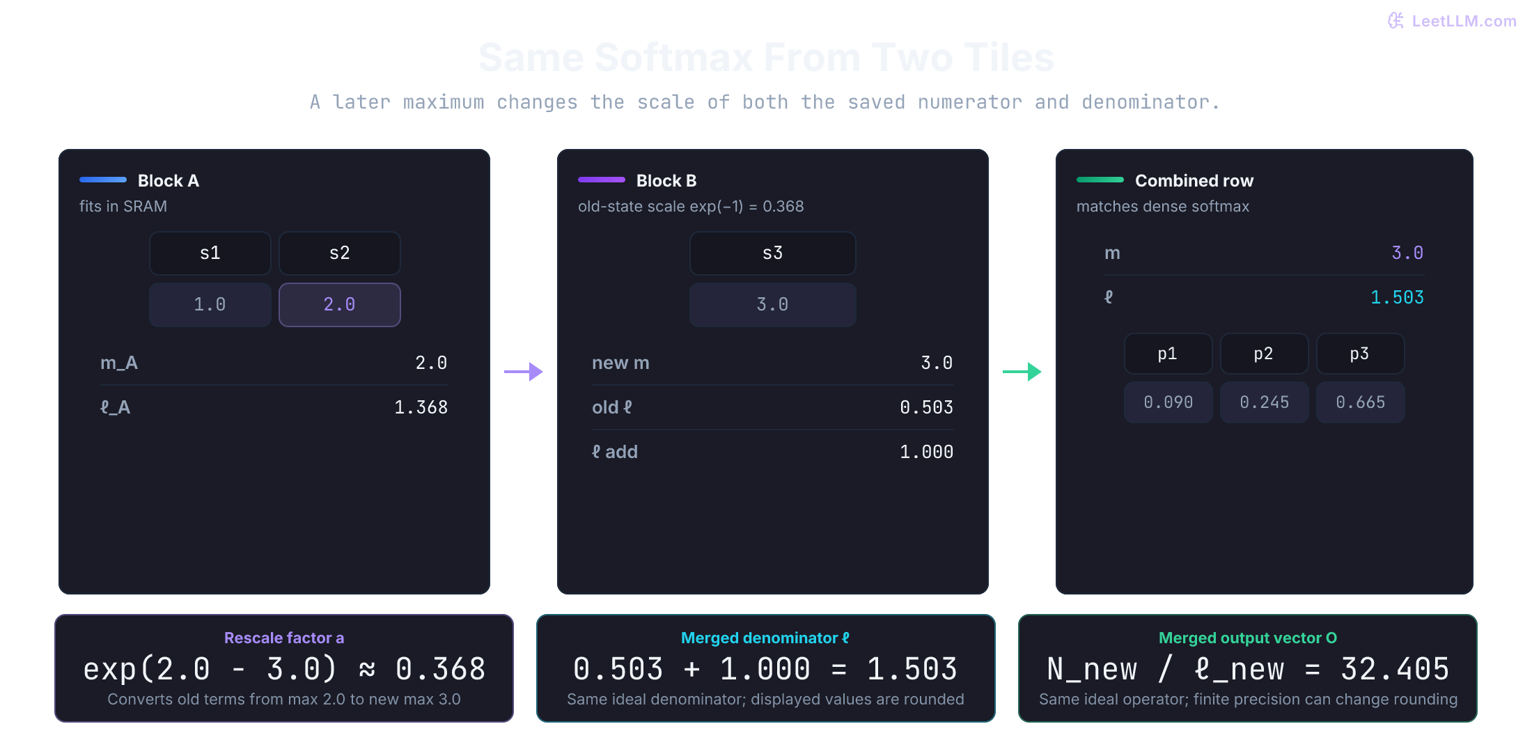
Test the same invariant with scalar values, independent of any GPU kernel:

import math

scores_a, values_a = [1.0, 2.0], [10.0, 20.0]
scores_b, values_b = [3.0], [40.0]

def local_state(scores, values):
    max_score = max(scores)
    weights = [math.exp(score - max_score) for score in scores]
    return max_score, sum(weights), sum(weight * value for weight, value in zip(weights, values))

m_a, l_a, n_a = local_state(scores_a, values_a)
m_b, l_b, n_b = local_state(scores_b, values_b)
m = max(m_a, m_b)
l = math.exp(m_a - m) * l_a + math.exp(m_b - m) * l_b
n = math.exp(m_a - m) * n_a + math.exp(m_b - m) * n_b
online = n / l

all_scores = scores_a + scores_b
all_values = values_a + values_b
dense_weights = [math.exp(score - max(all_scores)) for score in all_scores]
dense = sum(w * v for w, v in zip(dense_weights, all_values)) / sum(dense_weights)

print(f"online output: {online:.6f}")
print(f"dense output:  {dense:.6f}")
print(f"match: {abs(online - dense) < 1e-12}")
assert math.isclose(online, dense, abs_tol=1e-12)

online output: 32.404513
dense output:  32.404513
match: True

The general update rule

The two-block intuition scales to every row and every K/V tile. Here is the formal mathematical derivation of online softmax from first principles.

Recall the standard safe softmax for a row of scores $s \in \mathbb{R}^N$ and values $V \in \mathbb{R}^{N \times d}$:

$m = \max_{1 \le j \le N} s_j, \quad \ell = \sum_{j=1}^N e^{s_j - m}, \quad P_j = \frac{e^{s_j - m}}{\ell}, \quad O = \sum_{j=1}^N P_j V_j = \frac{\sum_{j=1}^N e^{s_j - m} V_j}{\ell}$

Now split the row into two blocks $s^{(1)}$ and $s^{(2)}$ with corresponding value slices $V^{(1)}$ and $V^{(2)}$:

• Block 1 has local max $m_1 = \max(s^{(1)})$, local denominator $\ell_1 = \sum_j e^{s^{(1)}_j - m_1}$, and unnormalized numerator $N_1 = \sum_j e^{s^{(1)}_j - m_1} V^{(1)}_j$.
• Block 2 has local max $m_2 = \max(s^{(2)})$, local denominator $\ell_2 = \sum_j e^{s^{(2)}_j - m_2}$, and unnormalized numerator $N_2 = \sum_j e^{s^{(2)}_j - m_2} V^{(2)}_j$.

To merge them without revisiting raw scores, identify the unified maximum:

$m_{\text{new}} = \max(m_1, m_2)$

We convert exponentials from base $m_1$ and $m_2$ to base $m_{\text{new}}$ using the identity:

$e^{s_j - m_{\text{new}}} = e^{(s_j - m) + (m - m_{\text{new}})} = e^{s_j - m} \cdot e^{m - m_{\text{new}}}$

Because $e^{m - m_{\text{new}}}$ is a scalar constant across all tokens in a block, pull it outside the sum:

$\sum_{j \in B_1} e^{s_j - m_{\text{new}}} = e^{m_1 - m_{\text{new}}} \sum_{j \in B_1} e^{s_j - m_1} = e^{m_1 - m_{\text{new}}} \cdot \ell_1$

The exact same algebra applies to the numerator sum:

$\sum_{j \in B_1} e^{s_j - m_{\text{new}}} V_j = e^{m_1 - m_{\text{new}}} \sum_{j \in B_1} e^{s_j - m_1} V_j = e^{m_1 - m_{\text{new}}} \cdot N_1$

Defining the rescale factors $a_1 = e^{m_1 - m_{\text{new}}}$ and $a_2 = e^{m_2 - m_{\text{new}}}$, the combined quantities are:

$\ell_{\text{new}} = a_1 \ell_1 + a_2 \ell_2$

$N_{\text{new}} = a_1 N_1 + a_2 N_2$

$O_{\text{new}} = \frac{N_{\text{new}}}{\ell_{\text{new}}}$

When processing tiles sequentially in a loop, block 1 represents the accumulated running state ($m_{\text{old}}, \ell_{\text{old}}, N_{\text{old}}$) and block 2 is the incoming score tile $s_{\text{tile}}$ and value tile $V_{\text{tile}}$. Then $m_{\text{new}} = \max(m_{\text{old}}, \max(s_{\text{tile}}))$, the old-state rescale factor is $a = e^{m_{\text{old}} - m_{\text{new}}}$, and the new weights are $p_j = e^{s_j - m_{\text{new}}}$. Here $d$ remains the head dimension; $\ell$ is the softmax denominator.

This reveals an important difference between FlashAttention versions:

• FlashAttention-1 kept the running output $O$ in normalized form at every step: $O_{\text{new}} = \frac{a \cdot \ell_{\text{old}}}{\ell_{\text{new}}} O_{\text{old}} + \frac{1}{\ell_{\text{new}}} \sum_j p_j V_j$ This normalizes the running output on every inner step.
• FlashAttention-2 keeps the accumulator in unnormalized form $O^* = N = \ell \cdot O$ throughout the inner loop: $O^*_{\text{new}} = a \cdot O^*_{\text{old}} + \sum_j p_j V_j$ The numerator update avoids repeated normalization. Softmax still needs maxima, exponentials, and sums. Once all K/V tiles have contributed, the kernel normalizes just once before writing $O$ to HBM: $O = \frac{O^*_{\text{final}}}{\ell_{\text{final}}}$ This reduces non-matmul overhead; it doesn't guarantee peak tensor-core throughput.^{[6]Reference 6FlashAttention-2: Faster Attention with Better Parallelism and Work Partitioning.https://arxiv.org/abs/2307.08691}

The saved LSE statistic is $L = m + \log \ell$, so backward can reconstruct a probability as $P_{ij} = e^{s_{ij} - L_i}$. Initialize the running state with $m = -\infty$, $\ell = 0$, and $N = 0$. Fully masked tiles need care: evaluating $-\infty - (-\infty)$ produces NaN. The sketch below handles those contributions explicitly. An entirely masked row has no mathematical softmax; returning zero matches the CPU PyTorch 2.14 behavior tested here and the FlashAttention package's documented convention.^{[7]Reference 7FlashAttentionhttps://github.com/Dao-AILab/flash-attention}

The equations establish equivalence in ideal arithmetic. The hardware schedule dictates where $Q, K, V,$ and running state reside. Later Q-resident schedules can write each final output tile and row statistic once. The original FA1 schedule also writes intermediate running state to HBM; both avoid the full $n\times n$ matrices.

Pseudocode

Now connect the state update to a hardware schedule. The original FlashAttention paper loops over K/V tiles in the outer loop and writes each Q tile's running state back to HBM between inner steps.^{[1]Reference 1FlashAttention: Fast and Memory-Efficient Exact Attention with IO-Awareness.https://arxiv.org/abs/2205.14135} FlashAttention-2 keeps a Q tile on-chip and streams K/V tiles past it, which cuts extra HBM traffic for $O$ and the row stats.^{[6]Reference 6FlashAttention-2: Faster Attention with Better Parallelism and Work Partitioning.https://arxiv.org/abs/2307.08691} The sketch below follows that later loop nest.

Read this as a single-head CPU correctness sketch, not a fused GPU kernel or a memory-efficient training implementation. It uses FP64 to compare the recurrence against PyTorch SDPA. Autograd retains intermediate operations here; FlashAttention's custom backward instead recomputes them. Boolean mask entries mean allowed, and Q/K lengths may differ.

import math
import torch
import torch.nn.functional as F

torch.set_num_threads(1)

def tiled_attention(q, k, v, allowed, block_size):
    if type(block_size) is not int or block_size <= 0:
        raise ValueError("block_size must be a positive integer")
    if any(x.ndim != 2 or x.dtype != torch.float64
           or x.device.type != "cpu" or not torch.isfinite(x).all()
           for x in (q, k, v)):
        raise ValueError("use finite 2D CPU float64 inputs")
    nq, d = q.shape
    nk, dk = k.shape
    if min(nq, nk, d, v.shape[1]) == 0 or d != dk or v.shape[0] != nk:
        raise ValueError("incompatible or empty Q/K/V shapes")
    if (allowed.shape != (nq, nk) or allowed.dtype != torch.bool
            or allowed.device.type != "cpu"):
        raise ValueError("allowed must be a boolean Q-length by K-length mask")
    outputs = []
    for i in range(0, nq, block_size):
        qi = q[i:i + block_size]
        m = torch.full((len(qi), 1), -torch.inf, dtype=q.dtype)
        l = torch.zeros_like(m)
        numerator = torch.zeros((len(qi), v.shape[1]), dtype=q.dtype)
        for j in range(0, nk, block_size):
            scores = qi @ k[j:j + block_size].T / math.sqrt(d)
            if not torch.isfinite(scores).all():
                raise ValueError("score arithmetic overflowed")
            scores = scores.masked_fill(~allowed[i:i + len(qi), j:j + block_size], -torch.inf)
            new_m = torch.maximum(m, scores.amax(dim=1, keepdim=True))
            # No valid key yet: use 0 as a temporary reference, avoiding -inf - -inf.
            reference = torch.where(torch.isfinite(new_m), new_m, 0.0)
            old_scale = torch.exp(m - reference)
            weights = torch.exp(scores - reference)
            numerator = old_scale * numerator + weights @ v[j:j + block_size]
            l = old_scale * l + weights.sum(dim=1, keepdim=True)
            if not torch.isfinite(numerator).all() or not torch.isfinite(l).all():
                raise ValueError("accumulator arithmetic overflowed")
            m = new_m
        # An empty row has zero numerator; divide it by 1, not 0.
        outputs.append(numerator / torch.where(l > 0, l, 1.0))
    return torch.cat(outputs)

torch.manual_seed(7)
q = torch.randn(5, 4, dtype=torch.float64, requires_grad=True)
k = torch.randn(7, 4, dtype=torch.float64, requires_grad=True)
v = torch.randn(7, 3, dtype=torch.float64, requires_grad=True)
# Five new queries after two cached positions: global query positions 2..6.
allowed = torch.arange(7)[None, :] <= (torch.arange(5) + 2)[:, None]
allowed[0] = False  # Exercise an entirely masked row as well as masked tiles.
expected = F.scaled_dot_product_attention(q, k, v, attn_mask=allowed, dropout_p=0.0)
reference_grads = torch.autograd.grad(expected.square().sum(), (q, k, v))
for block_size in (1, 3, 20):
    got = tiled_attention(q, k, v, allowed, block_size)
    torch.testing.assert_close(got, expected, atol=1e-12, rtol=1e-12)
    grads = torch.autograd.grad(got.square().sum(), (q, k, v))
    for actual, reference in zip(grads, reference_grads):
        torch.testing.assert_close(actual, reference, atol=1e-11, rtol=1e-11)
    assert torch.equal(got[0], torch.zeros(3, dtype=q.dtype))
    print(f"block={block_size}: output, gradients, and empty row match CPU SDPA")
large_q = torch.ones(1, 1, dtype=torch.float64)
large_k = torch.tensor([[1000.], [1001.], [-1000.]], dtype=torch.float64)
large_v = torch.tensor([[10.], [20.], [40.]], dtype=torch.float64)
mask = torch.ones(1, 3, dtype=torch.bool)
torch.testing.assert_close(
    tiled_attention(large_q, large_k, large_v, mask, 1),
    F.scaled_dot_product_attention(large_q, large_k, large_v),
    atol=1e-12, rtol=1e-12,
)
print("large-magnitude scores remain stable")
for invalid in (0, -1, 1.5, True):
    try:
        tiled_attention(q, k, v, allowed, invalid)
    except ValueError:
        pass
    else:
        raise AssertionError("invalid block size accepted")
print("invalid block sizes rejected")

block=1: output, gradients, and empty row match CPU SDPA
block=3: output, gradients, and empty row match CPU SDPA
block=20: output, gradients, and empty row match CPU SDPA
large-magnitude scores remain stable
invalid block sizes rejected

numerator stays unnormalized until every K/V tile for that Q block has contributed. The check covers unequal sequence lengths, a value dimension different from the query dimension, remainder tiles, masked tiles, an empty row, and gradients with respect to Q/K/V. None of those CPU checks measures GPU memory use or kernel speed.

Finite inputs do not guarantee finite intermediate arithmetic. Two very large values can overflow the unnormalized numerator even when their normalized mean fits in FP64. This sketch should reject that case rather than return infinity:

q_extreme = torch.zeros(1, 1, dtype=torch.float64)
k_extreme = torch.zeros(2, 1, dtype=torch.float64)
v_extreme = torch.full((2, 1), 1e308, dtype=torch.float64)
allow_all = torch.ones(1, 2, dtype=torch.bool)
dense_extreme = F.scaled_dot_product_attention(
    q_extreme, k_extreme, v_extreme, attn_mask=allow_all, dropout_p=0.0
)
assert torch.isfinite(dense_extreme).all()
print("normalized dense result is finite: True")
try:
    tiled_attention(q_extreme, k_extreme, v_extreme, allow_all, 2)
except ValueError as error:
    assert str(error) == "accumulator arithmetic overflowed"
    print("unnormalized accumulator overflow rejected")
else:
    raise AssertionError("silent overflow accepted")

normalized dense result is finite: True
unnormalized accumulator overflow rejected

Common mistake: Dividing numerator inside this loop without changing the recurrence mixes normalized and unnormalized state. A normalized running-output formulation is valid too, but its merge rule must restore the old denominator's weight. FlashAttention-1 uses such a formulation; normalization itself isn't the error.^{[1]Reference 1FlashAttention: Fast and Memory-Efficient Exact Attention with IO-Awareness.https://arxiv.org/abs/2205.14135}

Production kernels implement the same algebra much more aggressively, while also handling batching, multiple heads, masks, and dropout.

The backward pass: recomputation can win

Training introduces an even harsher memory bottleneck: backpropagation needs attention scores and probabilities to compute gradients with respect to $Q$, $K$, and $V$.

To see why, trace a materializing attention backward pass with dropout disabled and value dimension $d$. Forward computes $S = QK^T / \sqrt{d}$, $P = \operatorname{softmax}(S)$, and $O = PV$. Given the upstream output gradient $dO \in \mathbb{R}^{N \times d}$, calculus gives the gradients:

$dV = P^T dO$

$dP = dO V^T$

$dS = P \odot (dP - D), \quad \text{where } D_i = \sum_{k=1}^d dO_{ik} O_{ik} = dO_i \cdot O_i$

$dQ = \frac{dS K}{\sqrt{d}}, \quad dK = \frac{dS^T Q}{\sqrt{d}}$

Why can the softmax correction use $O$ instead of saving $dP$? For each row, $\sum_j P_{ij}dP_{ij}=\sum_j P_{ij}(dO_i\cdot V_j)=dO_i\cdot\sum_j P_{ij}V_j=dO_i\cdot O_i$. That identity reduces the correction to one scalar per query row.^{[1]Reference 1FlashAttention: Fast and Memory-Efficient Exact Attention with IO-Awareness.https://arxiv.org/abs/2205.14135} If values have width $d_v$ different from Q/K width $d$, this dot product runs over $d_v$; the score scale still uses $\sqrt d$.

Check the equations directly on the sketch's unequal-length masked inputs. This dense diagnostic deliberately materializes probabilities. It also gives an empty row zero probabilities and gradients, matching the explicit convention used above.

with torch.no_grad():
    scores = (q @ k.T / math.sqrt(q.shape[1])).masked_fill(~allowed, -torch.inf)
    row_max = scores.amax(dim=1, keepdim=True)
    reference = torch.where(torch.isfinite(row_max), row_max, 0.0)
    weights = torch.exp(scores - reference)
    denominator = weights.sum(dim=1, keepdim=True)
    p = weights / torch.where(denominator > 0, denominator, 1.0)
    output = p @ v
    upstream = torch.arange(output.numel(), dtype=q.dtype).reshape_as(output) / 10
    dp = upstream @ v.T
    correction = (upstream * output).sum(dim=1, keepdim=True)
    torch.testing.assert_close(correction, (p * dp).sum(dim=1, keepdim=True))
    ds = p * (dp - correction)
    manual = (ds @ k / math.sqrt(q.shape[1]),
              ds.T @ q / math.sqrt(q.shape[1]), p.T @ upstream)

reference_output = F.scaled_dot_product_attention(q, k, v, attn_mask=allowed, dropout_p=0.0)
automatic = torch.autograd.grad((reference_output * upstream).sum(), (q, k, v))
for name, actual, expected in zip(("Q", "K", "V"), manual, automatic):
    torch.testing.assert_close(actual, expected, atol=1e-12, rtol=1e-12)
    print(f"manual d{name} matches SDPA autograd")
assert torch.equal(manual[0][0], torch.zeros_like(q[0]))
print("empty query row contributes zero gradient")

manual dQ matches SDPA autograd
manual dK matches SDPA autograd
manual dV matches SDPA autograd
empty query row contributes zero gradient

One baseline saves the entire probability matrix $P$ during forward and reads it during backward; the gradient equations don't require saving $S$ as well. Our FP16 example uses 32 GiB to store $P$, and 64 GiB for one write plus one read. Keeping one such matrix for each of 32 layers would occupy 1 TiB. Sharding, offloading, or recomputation can change that storage requirement; an immediate crash isn't inevitable.

FlashAttention avoids saving full $P$ and $S$.^{[1]Reference 1FlashAttention: Fast and Memory-Efficient Exact Attention with IO-Awareness.https://arxiv.org/abs/2205.14135} Modern implementations retain references to existing $Q, K, V$, save $O$, and write a compact row statistic $L_i = m_i + \log \ell_i$ for backward. The attention kernel doesn't need to rewrite its input tensors merely to retain them. Dropout-enabled paths also retain state needed to reproduce the random mask. The original FA1 algorithm stores the pair $(m,\ell)$; the current package saves their combined LSE representation.^{[1]Reference 1FlashAttention: Fast and Memory-Efficient Exact Attention with IO-Awareness.https://arxiv.org/abs/2205.14135[7]Reference 7FlashAttentionhttps://github.com/Dao-AILab/flash-attention}

For our batch/head/sequence configuration, FP32 $L$ takes 8 MiB, compared to 32 GiB for one FP16 probability matrix. The 4,096× ratio compares those two arrays, not all saved activations or total GPU memory. Q/K/V/O remain.

During the backward pass, FlashAttention recomputes the score and probability tiles directly on-chip in SRAM:

1. It loads a tile of $Q_i, K_j, V_j, dO_i,$ and the scalars $L_i$ into SRAM.
2. It recomputes the local score tile on-chip: $S_{ij} = Q_i K_j^T / \sqrt{d}$.
3. Using the saved statistic $L_i$, it recovers the exact probabilities on-the-fly in SRAM registers: $P_{ij} = \exp(S_{ij} - L_i)$
4. It immediately evaluates the gradient equations on-chip, accumulating into $dQ, dK,$ and $dV$, and throws the intermediate $S_{ij}$ and $P_{ij}$ tiles away.

Recomputing tiles adds arithmetic but avoids transferring the saved quadratic array. That trade can reduce runtime when the avoided traffic costs more than the extra computation. Tile dimensions alone don't establish either time: head dimension, dtype, scheduling, and GPU matter. The auxiliary-memory saving follows from which arrays are retained; a backward speedup still needs measurement.

This calculator compares one FP16 probability matrix with the FP32 softmax_lse tensor saved by the current flash-attention interface, not every tensor in training:

batch, heads, sequence = 8, 32, 8192
materialized_probabilities = batch * heads * sequence * sequence * 2
softmax_lse = batch * heads * sequence * 4

print(f"one saved probability matrix: {materialized_probabilities / 1024**3:.2f} GiB")
print(f"FP32 softmax LSE:        {softmax_lse / 1024**2:.2f} MiB")
print(f"size ratio:             {materialized_probabilities / softmax_lse:,.0f}x")
print(f"one write plus one read: {2 * materialized_probabilities / 1024**3:.2f} GiB")

one saved probability matrix: 32.00 GiB
FP32 softmax LSE:        8.00 MiB
size ratio:             4,096x
one write plus one read: 64.00 GiB

Complexity analysis

With the mechanism in hand, separate mathematical work, extra attention state, and memory traffic. In the paper's two-level memory model, $M$ is fast-memory capacity measured in scalar elements, not bytes, and the stated bound assumes $d \leq M \leq nd$. Batch and head count are held fixed. The linear-memory shorthand also holds head dimension $d$ fixed.

FLOPs stands for floating-point operations. The memory row refers to extra state created by the attention kernel itself, not the shared $Q$, $K$, $V$, and $O$ tensors that both approaches still need to hold.

FlashAttention doesn't reduce the asymptotic mathematical work: both paths still do $O(n^2 d)$ operations. The win is avoiding $n^2$ score and probability transfers through HBM. Tile size, scheduling, datatype, and hardware still change observed speed.

Under the paper's SRAM model, tiling changes HBM reads and writes from $\Theta(nd + n^2)$ for the materializing baseline to $\Theta(n^2 d^2 / M)$.^{[1]Reference 1FlashAttention: Fast and Memory-Efficient Exact Attention with IO-Awareness.https://arxiv.org/abs/2205.14135} A larger usable SRAM budget $M$ lets each tile reuse more data before returning to HBM. This is an IO-model result, not a wall-clock guarantee: both paths still perform $O(n^2 d)$ arithmetic, and kernel schedules determine how much of the bound appears in a benchmark.

With fixed hardware capacity $M$ and fixed head dimension $d$, the IO expression still grows quadratically in sequence length. Linear auxiliary storage means no full score/probability array is retained; it doesn't mean linear total data movement.

Because FlashAttention computes the same dense operator (via online softmax), it doesn't change the model's attention rule. Different floating-point association can still cause small numeric differences.

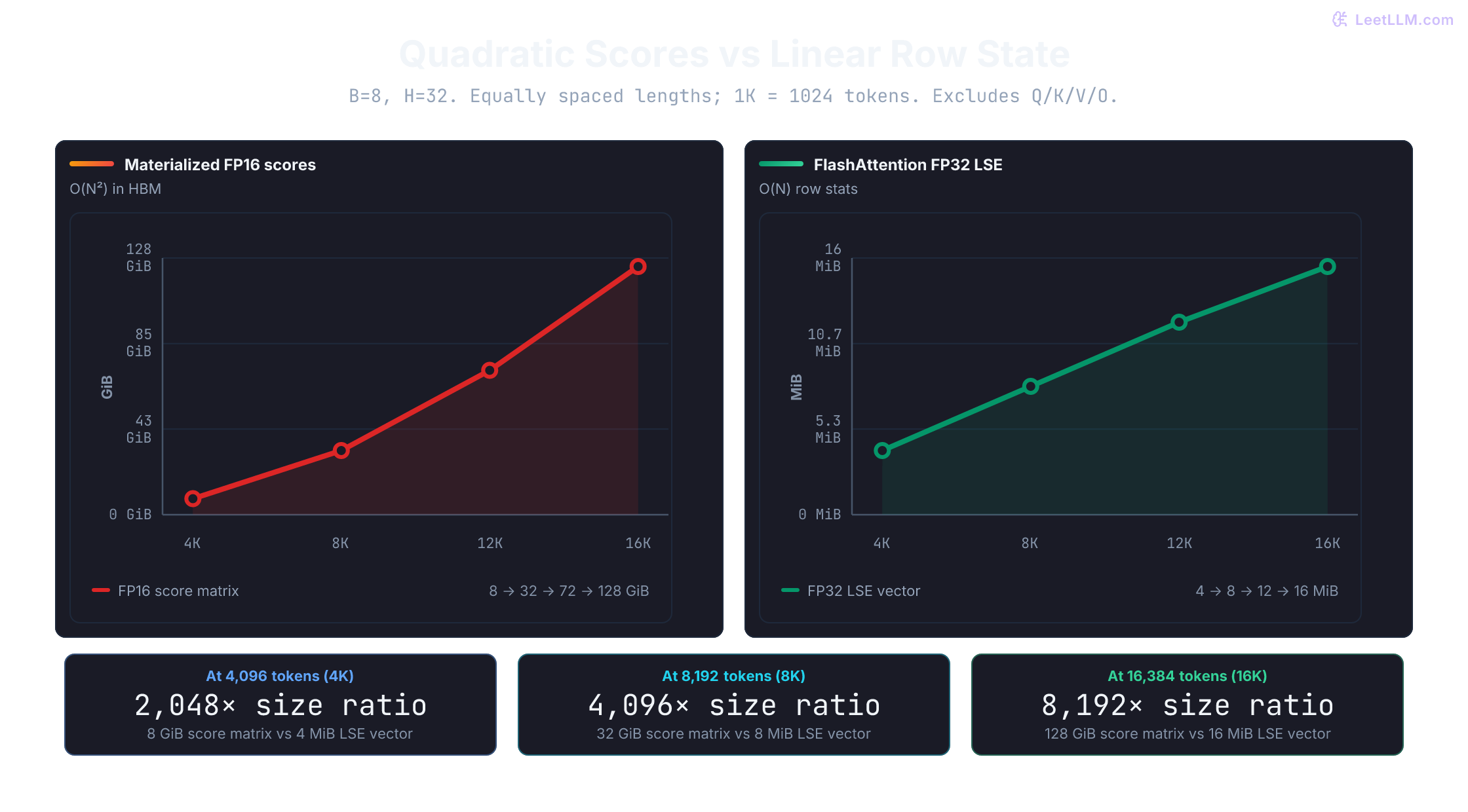
Predict the curves before running the small scaling check: a score matrix should grow with the square of sequence length, while one row statistic per token should grow linearly.

These numbers distinguish score-matrix scaling from row-statistic scaling:

base_sequence = 1024
for sequence in [1024, 2048, 4096, 8192, 16384]:
    materialized_relative = (sequence / base_sequence) ** 2
    row_stats_relative = sequence / base_sequence
    print(
        f"{sequence:>5} tokens: materialized={materialized_relative:>5.0f}x, "
        f"row-stats={row_stats_relative:>2.0f}x"
    )

1024 tokens: materialized=    1x, row-stats= 1x
 2048 tokens: materialized=    4x, row-stats= 2x
 4096 tokens: materialized=   16x, row-stats= 4x
 8192 tokens: materialized=   64x, row-stats= 8x
16384 tokens: materialized=  256x, row-stats=16x

Causal masking in FlashAttention

For autoregressive transformers, attention is causal: token $i$ can only attend to tokens $j \leq i$. A materializing baseline allocates a full $N \times N$ matrix and masks the upper triangle. At 8,192 tokens, over 33.5 million entries per head represent invalid future pairs, yet the full allocation remains.

FlashAttention handles causal attention without materializing any causal mask tensor in HBM. The mask becomes part of the tiled kernel schedule.

Block-level skipping

First assume square self-attention, equal aligned tile sizes $B_r=B_c=B$, and $N$ divisible by $B$. This creates a $T\times T$ grid with $T=N/B$. For query tile $i$ and key tile $j$:

1. Upper-triangular tiles ($j > i$): Every key is future context for every query. The scheduler can omit this pair's matrix multiplication and value contribution. Actual prefetching and memory allocation depend on the implementation; skipping a pair doesn't prove that its K/V block is never loaded for another query tile.
2. Lower-triangular tiles ($j < i$): Every key is valid past context. No per-element causal mask is needed, though padding or other constraints may still apply.
3. Diagonal tiles ($j = i$): The query and key tiles overlap in sequence position. The kernel computes the tile dot products $S_{ij} = Q_i K_j^T / \sqrt{d}$ in SRAM, then applies an in-SRAM causal mask: entries where intra-tile key index exceeds intra-tile query index are set to $-\infty$ before the online softmax update.

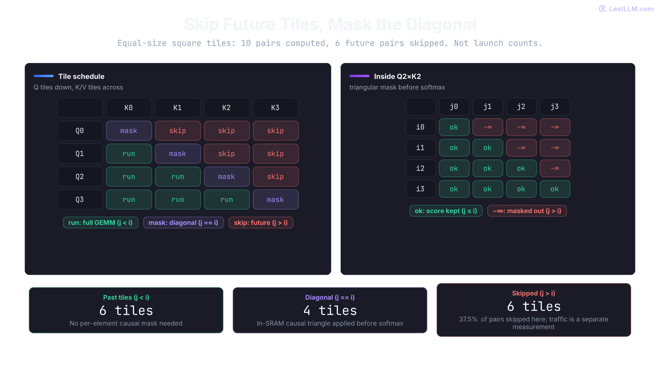
Counting skipped tile work

In a $T \times T$ tile grid, total tile pairs equal $T^2$. Count the workload:

• Strictly past tiles ($j < i$): $\frac{T(T-1)}{2}$
• Diagonal tiles ($j = i$): $T$
• Total tiles computed: $\frac{T(T+1)}{2}$
• Future tiles skipped ($j > i$): $\frac{T(T-1)}{2}$

As sequence length grows relative to tile size (large $T$), the fraction of tiles computed is:

$\frac{\text{Computed tiles}}{\text{Total tiles}} = \frac{T(T+1)}{2 T^2} = \frac{1}{2} + \frac{1}{2T} \xrightarrow{T \to \infty} 50\%$

In the four-tile figure, 10 of 16 pairs run: 62.5% computed, 37.5% skipped. The skipped fraction approaches 50% for a large equal-tile grid. That describes omitted tile work, not a guaranteed 50% reduction in physical K/V traffic or runtime. Cache reuse, diagonal work, buffering, and scheduling affect those separately.

You can audit causal tile decisions without any GPU code:

tiles = 4
counts = {"past": 0, "boundary": 0, "future": 0}

for query_tile in range(tiles):
    for key_tile in range(tiles):
        if key_tile < query_tile:
            decision = "past"
        elif key_tile == query_tile:
            decision = "boundary"
        else:
            decision = "future"
        counts[decision] += 1

print(counts)
print(f"computed tiles: {counts['past'] + counts['boundary']} of {tiles * tiles}")

{'past': 6, 'boundary': 4, 'future': 6}
computed tiles: 10 of 16

Unequal tile widths and cached query offsets break the shortcut $j>i$. Compare absolute position ranges instead: a tile is entirely future if its first key comes after its last query, entirely allowed if its last key is no later than its first query, and otherwise crosses the causal boundary.

def classify(query_start, query_end, key_start, key_end):
    if key_start > query_end:
        return "future"
    if key_end <= query_start:
        return "past"
    return "boundary"

# Query tile 1 of width 128 meets key tile 2 of width 64.
# The key tile index is larger, but some of its keys are still valid.
for key_start, key_end, expected in (
    (128, 191, "boundary"), (0, 127, "past"), (256, 319, "future")
):
    decision = classify(128, 255, key_start, key_end)
    assert decision == expected
    print(f"Q128..255 x K{key_start}..{key_end}: {decision}")

Q128..255 x K128..191: boundary
Q128..255 x K0..127: past
Q128..255 x K256..319: future

FlashAttention-2, FlashAttention-3, and FlashAttention-4

Once tiling eliminates full HBM matrix materialization, work partitioning, instruction scheduling, and hardware pipelines become the next performance bottlenecks. The core algorithm remains exact dense attention, but the hardware execution model has evolved across four distinct generations.

Generational comparison

FlashAttention-1: the IO-aware foundation

The original paper identified full-matrix materialization as an IO bottleneck in its baselines.^{[1]Reference 1FlashAttention: Fast and Memory-Efficient Exact Attention with IO-Awareness.https://arxiv.org/abs/2205.14135} It split $Q, K, V$ into SRAM-sized blocks and used online softmax to update row statistics incrementally. This doesn't establish that every attention kernel on every GPU is memory-bound.

However, FlashAttention-1 structured its loop nest with the outer loop over K/V blocks and the inner loop over Q blocks. Because Q blocks cycled in the inner loop, intermediate output accumulators and running softmax statistics were repeatedly saved back to HBM and reloaded across outer steps. On top of that, FA1 maintained a normalized running output at each step, forcing elementwise division operations inside every inner iteration.

FlashAttention-2: loop inversion and warp partitioning

FlashAttention-2 attacked GPU occupancy and non-matmul overhead:^{[6]Reference 6FlashAttention-2: Faster Attention with Better Parallelism and Work Partitioning.https://arxiv.org/abs/2307.08691}

1. Loop inversion: It flipped the loop nest so the outer loop iterates over Q blocks and the inner loop streams K/V blocks through SRAM. A Q block is loaded into fast SRAM registers once and remains pinned there until all K/V blocks have contributed. This cuts out intermediate HBM writes for the output accumulator.
2. Unnormalized accumulation: It maintains $O^* = \ell \cdot O$ and normalizes the output once at the end. The tile's exponentials are unnormalized weights, not independently normalized probabilities. Maxima, exponentials, sums, and rescaling still occur inside the loop.
3. Warp-level partitioning along Q: FA1's split-K scheme combines partial outputs through shared-memory writes, synchronization, and reduction. FA2 gives warps independent query rows, removing that output-combination step. This isn't a claim that the whole kernel needs no synchronization; its backward pass has additional dependencies.
4. Sequence-length parallelization: FA2 also assigns query blocks to separate thread blocks, increasing available parallelism when batch size and head count alone provide too little work. Resource limits still determine achieved occupancy.

On an A100, FlashAttention-2 reached 50-73% of theoretical peak, about 2× faster than FlashAttention-1, delivering up to 230 TFLOPs/s in FP16.^{[6]Reference 6FlashAttention-2: Faster Attention with Better Parallelism and Work Partitioning.https://arxiv.org/abs/2307.08691}

FlashAttention-3: Hopper TMA and warp specialization

On NVIDIA Hopper (H100), raw compute capacity grew faster than memory bandwidth. FlashAttention-3 redesigned the pipeline to exploit Hopper's architectural features:^{[8]Reference 8FlashAttention-3: Fast and Accurate Attention with Asynchrony and Low-precision.https://arxiv.org/abs/2407.08608}

1. Asynchronous memory transfers with TMA: A thread can issue a multidimensional copy between global and shared memory without staging each element through its registers. Issuing the copy and synchronizing its completion still require instructions.^{[3]Reference 3NVIDIA Hopper Tuning Guidehttps://docs.nvidia.com/cuda/hopper-tuning-guide/index.html}
2. Asynchronous tensor core math with WGMMA: A warpgroup (128 threads across 4 warps) coordinates matrix multiplication. FA3 uses both shared-memory and register-sourced first operands; the results and subsequent softmax still have dependencies.
3. Warp specialization: Producer warps issue copies while consumer warps perform compute. Circular buffers and barriers allow overlap where dependencies and resources permit it. They don't guarantee complete overlap of every transfer.
4. Interleaving softmax with GEMM: Pipelining can overlap softmax with independent matrix work, reducing exposed exponential latency. Extra buffers and synchronization are part of the trade-off.
5. Low-precision FP8: It adds a block-quantized FP8 forward path with incoherent processing techniques to handle outlier activations, reaching up to 740 TFLOPs/s in FP16 (75% utilization) and nearly 1.2 PFLOPs/s in FP8 on H100.^{[8]Reference 8FlashAttention-3: Fast and Accurate Attention with Asynchrony and Low-precision.https://arxiv.org/abs/2407.08608}

FlashAttention-4: Blackwell co-design and CuTe-DSL

The March 2026 paper addresses Blackwell's imbalance between fast tensor cores and slower exponential execution and shared-memory traffic.^{[9]Reference 9FlashAttention-4: Algorithm and Kernel Pipelining Co-Design for Asymmetric Hardware Scalinghttps://arxiv.org/abs/2603.05451} Three changes matter:

• Larger-tile asynchronous MMA pipelines overlap softmax with matrix work.
• Software-emulated exponentials and conditional rescaling reduce non-matmul overhead. When a maximum increase is small, the algorithm can keep the old reference maximum and evaluate all new weights against it. Numerator and denominator remain consistently scaled; simply forgetting to rescale while switching references would be wrong.
• Tensor memory and two-CTA backward execution reduce shared-memory traffic and global atomic additions.

The Python-embedded CuTe-DSL still compiles GPU kernels. The authors report much shorter compilation than their FA3 C++ template implementation, not an absence of compilation.

Their B200 BF16 kernel benchmarks report up to 1,613 TFLOPs/s (71% peak), 1.3× cuDNN 9.13, and 2.7× Triton. They vary causal/noncausal attention, head dimensions, and lengths 1K–32K with total tokens fixed at 32K. These are kernel results, not application throughput. The paper also notes that newer cuDNN versions incorporated related techniques and reached similar performance.^{[9]Reference 9FlashAttention-4: Algorithm and Kernel Pipelining Co-Design for Asymmetric Hardware Scalinghttps://arxiv.org/abs/2603.05451}

Measured performance

Training throughput

Treat benchmark rows as scoped evidence, not universal multipliers.

During model training, saving quadratic attention intermediates can sharply restrict the maximum sequence length a model can process. As sequence length increases, a materializing baseline may run out of memory even when a fused attention path can still fit.

Common mistake: Assuming FlashAttention is only a "long-sequence hack." The original paper reports a 15% end-to-end speedup for BERT-large at sequence length 512 on eight A100 GPUs against the MLPerf 1.1 implementation. Training to the target masked-language-model accuracy took 17.4 minutes versus 20.0 minutes, averaged over ten runs. That is a specific moderate-length workload, not a universal multiplier.^{[1]Reference 1FlashAttention: Fast and Memory-Efficient Exact Attention with IO-Awareness.https://arxiv.org/abs/2205.14135}

For each result below, keep workload, sequence length, hardware, and baseline attached to the number.

Compared with a baseline that saves full attention intermediates, FlashAttention's auxiliary attention memory grows linearly rather than quadratically. That can enable longer sequences and improve throughput even while a materializing baseline still fits in memory.^{[1]Reference 1FlashAttention: Fast and Memory-Efficient Exact Attention with IO-Awareness.https://arxiv.org/abs/2205.14135[6]Reference 6FlashAttention-2: Faster Attention with Better Parallelism and Work Partitioning.https://arxiv.org/abs/2307.08691}

Model FLOPs utilization is an end-to-end training metric, unlike the attention-kernel throughput reported in the preceding section. Don't compare the two as if they timed the same operation. A faster attention kernel may leave optimizer steps, communication, or feed-forward layers as the dominant cost.

Inference impact

During inference, FlashAttention helps most when the workload still looks like dense attention over many prompt tokens:

• Prefill has many query rows. In our coding-assistant example, each query scores itself and earlier keys. Avoiding quadratic intermediates can reduce memory pressure and the attention portion of time to first token (TTFT).
• Decode usually has one query per request and reuses the KV cache. Reading that cache can dominate attention time; at small batches, streaming model weights may dominate the whole step instead.
• Long prompts amplify the potential memory saving, but don't guarantee a larger application speedup. The baseline backend, batch, head dimensions, and active bottleneck all matter.

Training and prefill expose the full quadratic-intermediate problem. Decode has a different shape and benefits from kernels designed for it.

Production decode uses a related but distinct kernel contract

Serving engines rarely keep one contiguous KV tensor per request. PagedAttention stores K/V in blocks and maps logical positions through a block table. Production decode therefore needs kernels that apply FlashAttention-style tiling and online softmax over non-contiguous KV blocks, beyond the training and prefill dense path.

Examples of that contract (names and APIs evolve):

• The package's flash_attn_with_kvcache, whose documented paged layout requires a page size divisible by 256 and whose interface doesn't support backward^{[7]Reference 7FlashAttentionhttps://github.com/Dao-AILab/flash-attention}
• FlashInfer and engine-specific paged attention kernels used by stacks such as vLLM

Those kernels are complementary to the PagedAttention allocator: paging decides where blocks live and how they are shared; the kernel decides how Q attends to them. A 16-token allocator example isn't automatically compatible with an interface requiring 256-token pages. Verify the selected backend's layout and page-size contract. GQA/MQA further shrinks the cache. Measure prefill TTFT and decode ITL separately.

Count valid causal pairs separately from the full square workspace. Here a decode query sees 8,192 valid keys total, including its current position if present. These counts are per head, not measured kernel instruction counts:

prompt_tokens = 8192
prefill_scores = prompt_tokens * (prompt_tokens + 1) // 2
decode_scores = 1 * prompt_tokens

print(f"valid causal prefill pairs: {prefill_scores:,}")
print(f"one decode step scores: {decode_scores:,}")
print(f"pair-count ratio: {prefill_scores / decode_scores:,.1f}x")

valid causal prefill pairs: 33,558,528
one decode step scores: 8,192
pair-count ratio: 4,096.5x

Hardware compatibility

Generation names are not dispatch guarantees. FA3 targets Hopper's TMA, WGMMA, and FP8 features.^{[8]Reference 8FlashAttention-3: Fast and Accurate Attention with Asynchrony and Low-precision.https://arxiv.org/abs/2407.08608} FA4's paper benchmarks Blackwell, while the current repository's CuTe implementation targets both Hopper and Blackwell.^{[7]Reference 7FlashAttentionhttps://github.com/Dao-AILab/flash-attention} Paper hardware and current package compatibility aren't the same list.

Availability in an application depends on its framework build, device, datatype, tensor shapes, and attention features. Treat backend selection as something to verify, not something to infer from the model name.

Using FlashAttention in practice

In modern deep learning frameworks, you rarely implement FlashAttention from scratch. PyTorch exposes torch.nn.functional.scaled_dot_product_attention (SDPA), which may choose an optimized CUDA implementation when the inputs and build support it. Its sdpa_kernel context manager lets you select permitted implementations while testing or profiling. Eligibility and fallback behavior depend on the installed PyTorch build, device, datatype, layout, and attention features, so consult the documentation for that build and measure the actual path.^{[2]Reference 2torch.nn.functional.scaled_dot_product_attentionhttps://docs.pytorch.org/docs/2.14/generated/torch.nn.functional.scaled_dot_product_attention.html}

Keep three claims separate: the operator is correct, the requested backend was selected, and the workload got faster. The next checks test them in that order.

First check the causal operator on a tiny row, in plain Python. This is the math SDPA is supposed to implement, not a FlashAttention dispatch test. Query token 1 may see keys 0 and 1 only:

import math

scores = [1.0, 2.0, 0.5, 3.0]
values = [10.0, 20.0, 40.0, 80.0]

def weighted_sum(scores, values, allowed):
    masked = [score if ok else float("-inf") for score, ok in zip(scores, allowed)]
    max_score = max(masked)
    weights = [
        0.0 if score == float("-inf") else math.exp(score - max_score)
        for score in masked
    ]
    total = sum(weights)
    return sum(weight * value for weight, value in zip(weights, values)) / total

causal = weighted_sum(scores, values, [True, True, False, False])
full = weighted_sum(scores, values, [True, True, True, True])
print(f"causal output: {causal:.6f}")
print(f"full output:   {full:.6f}")
print(f"masking changed the blend: {causal != full}")

causal output: 17.310586
full output:   58.029621
masking changed the blend: True

Causal masking changes the blend because score 3.0 is future context for query 1. For equal query/key lengths, is_causal=True applies that lower-triangular rule. Unequal lengths need more care: PyTorch SDPA aligns this mask to the upper left, while the FlashAttention package changed to bottom-right alignment in version 2.1.^{[2]Reference 2torch.nn.functional.scaled_dot_product_attentionhttps://docs.pytorch.org/docs/2.14/generated/torch.nn.functional.scaled_dot_product_attention.html[7]Reference 7FlashAttentionhttps://github.com/Dao-AILab/flash-attention} Swapping APIs without checking that convention can change model outputs.

For one query against four already-valid cache entries, upper-left causal masking admits only the first key. Equal scores make the mistake easy to see: the correct output averages all four values. For a chunk of new queries, build a mask from absolute query/key positions, as the tiled sketch did.

import torch
import torch.nn.functional as F

torch.set_num_threads(1)

q = torch.zeros(1, 1, 1, 2, dtype=torch.float64)
k = torch.zeros(1, 1, 4, 2, dtype=torch.float64)
v = torch.tensor([10., 20., 40., 80.], dtype=torch.float64).reshape(1, 1, 4, 1)
upper_left = F.scaled_dot_product_attention(q, k, v, is_causal=True, dropout_p=0.0)
# All four cache entries are valid for this query, so no causal mask is needed.
valid_cache = F.scaled_dot_product_attention(q, k, v, is_causal=False, dropout_p=0.0)
assert upper_left.item() == 10.0
assert valid_cache.item() == 37.5
print(f"upper-left causal output: {upper_left.item():.1f}")
print(f"all-valid cache output:   {valid_cache.item():.1f}")

upper-left causal output: 10.0
all-valid cache output:   37.5

Padding, unused cache capacity, or future keys still require masking. Setting is_causal=False is correct here only because every supplied key is valid.

Once the math is right, test dispatch. On CUDA, sdpa_kernel(SDPBackend.FLASH_ATTENTION) restricts the permitted backend. Unsupported inputs may raise an error; the restricted context doesn't silently fall back to math.^{[2]Reference 2torch.nn.functional.scaled_dot_product_attentionhttps://docs.pytorch.org/docs/2.14/generated/torch.nn.functional.scaled_dot_product_attention.html} Check eligibility first with can_use_flash_attention, including the same mask, dropout, causal, and GQA settings as the actual call.^{[10]Reference 10torch.backends.cuda: SDPA backend eligibilityhttps://docs.pytorch.org/docs/stable/backends.html} This GPU-only example lets execution errors propagate instead of misclassifying every RuntimeError as an unsupported backend.

import torch
import torch.nn.functional as F
from torch.nn.attention import SDPBackend, sdpa_kernel
from torch.backends.cuda import SDPAParams, can_use_flash_attention

Q = torch.randn(2, 16, 1024, 64, device="cuda", dtype=torch.float16)
K = torch.randn(2, 16, 1024, 64, device="cuda", dtype=torch.float16)
V = torch.randn(2, 16, 1024, 64, device="cuda", dtype=torch.float16)

def attention_with_flash_probe(Q, K, V):
    params = SDPAParams(Q, K, V, None, 0.0, True, False)
    if can_use_flash_attention(params, debug=True):
        with sdpa_kernel(SDPBackend.FLASH_ATTENTION):
            output = F.scaled_dot_product_attention(
                Q, K, V, is_causal=True, dropout_p=0.0
            )
        return output, "restricted_flash_completed"
    print("FlashAttention ineligible; using the default permitted backends.")
    output = F.scaled_dot_product_attention(
        Q, K, V, is_causal=True, dropout_p=0.0
    )
    return output, "default_backend_selection"

output, dispatch_path = attention_with_flash_probe(Q, K, V)
print("dispatch policy:", dispatch_path)

An out-of-memory error or device failure isn't evidence of backend ineligibility, and a math fallback may need more memory. Successful restriction establishes that a permitted implementation ran, not that it beat the default or selected FA4. Record the PyTorch/CUDA versions, GPU, shapes, mask, dtype, and profiler trace. Warm up both paths, synchronize CUDA timing, and compare repeated latency samples plus peak allocated memory on identical inputs.^{[11]Reference 11Accelerating PyTorch 2 Transformers with torch.compile and scaled_dot_product_attentionhttps://docs.pytorch.org/tutorials/intermediate/scaled_dot_product_attention_tutorial.html} Set dropout_p=0.0 explicitly at inference; SDPA doesn't inspect a module's .eval() state.^{[2]Reference 2torch.nn.functional.scaled_dot_product_attentionhttps://docs.pytorch.org/docs/2.14/generated/torch.nn.functional.scaled_dot_product_attention.html}

Current Transformers backends accept attn_implementation="flash_attention_2" or "flash_attention_3" as a load-time request and can also load supported Hub kernels.^{[12]Reference 12Transformers: Attention Backendshttps://huggingface.co/docs/transformers/en/attention_interface} Check model support and dependency compatibility. The string is a request, not a profiler trace:

import torch
from transformers import AutoModelForCausalLM

model = AutoModelForCausalLM.from_pretrained(
    "your-org/your-supported-causal-lm",
    dtype=torch.bfloat16,
    attn_implementation="flash_attention_2",
    device_map="auto",
)

For direct FA4 use, the current repository documents installing flash-attn-4 and importing flash_attn_func from flash_attn.cute.^{[7]Reference 7FlashAttentionhttps://github.com/Dao-AILab/flash-attention} That is a separate package path, not a version automatically selected by PyTorch's FLASH_ATTENTION enum. Check the repository's current CUDA/GPU requirements and the function's layout contract before integrating it.

Common mistakes

"FlashAttention is an approximation"

If you group FlashAttention with sparse or low-rank methods, you'll explain the memory saving incorrectly. Tiling preserves the dense formula rather than dropping allowed connections. Compare outputs and gradients with a reference at the intended dtype; the FP64 CPU check establishes the recurrence, not the accuracy of an FP8 GPU implementation.

"FlashAttention reduces the number of compute operations"

An $O(n)$ memory label doesn't imply linear compute. Dense attention still performs $O(n^2d)$ arithmetic; causal skipping changes its constant factor, not that order. Backward recomputation adds work. When explaining a speedup, identify the avoided transfers and the baseline instead of treating “faster” as evidence of fewer FLOPs.

"GPU memory is one big pool"

An 80 GB device doesn't provide an 80 GB tile workspace. Check per-SM shared memory, register pressure, accumulator precision, and overlapping load buffers. Our 144 KiB logical subtotal isn't a legal launch configuration by itself. Likewise, the 8 MiB LSE statistic isn't total training memory: Q/K/V/O and the rest of the model remain.

"A backend swap preserves my mask automatically"

If cached decoding suddenly changes outputs, inspect absolute query positions and causal alignment before blaming floating-point error. The one-query example returns 10 instead of 37.5 under an upper-left mask. Check padding and unused cache slots too. Then verify dropout and compare the operator before profiling the replacement backend.