Reward Modeling from Preference Data

A pairwise reward model learns to score completed responses from preference comparisons. Unlike supervised fine-tuning (SFT), which trains a network to imitate demonstration tokens, reward modeling fits an evaluative judge that separates preferred answers from rejected ones.

Consider an access-policy assistant in an enterprise setting. Company policy P-7 requires an approved access-review ticket before granting production database credentials. A user submits an urgent request during a database migration. One completion follows rule P-7 by opening a ticket and citing policy; a second grants admin access immediately to appear helpful. A third follows the rule but pads the response with three paragraphs of apologetic disclaimers. If the evaluative judge rewards raw length or deferential tone rather than policy compliance, it'll favor the wrong response. We'll use this running access-policy example to separate learning genuine human preference from picking up superficial training shortcuts.

System diagrams for RLHF (Reinforcement Learning from Human Feedback) often compress this pipeline into a box labeled reward model, before jumping to Proximal Policy Optimization (PPO). In the scalar-model recipe, that box is a neural network trained on noisy comparisons.^{[1]Reference 1Training Language Models to Follow Instructions with Human Feedback (InstructGPT).https://arxiv.org/abs/2203.02155} If it learns a shortcut such as verbosity, policy optimization can amplify the mistake.^{[2]Reference 2Scaling Laws for Reward Model Overoptimizationhttps://proceedings.mlr.press/v202/gao23h.html} We'll build the judge, inspect its gradients, and try to fool it before using it to train a generator.

A scalar judge, not a generator

This lesson trains a scalar reward model. Generative judges also exist, but the head we build here returns a score. An autoregressive language model instead computes a conditional probability distribution over the vocabulary $V$ at each step:

$$\pi_\theta(y_t \mid x, y_{<t}) \in \Delta^{|V|-1}$$

A reward model, by contrast, acts as a sequence scorer. It ingests a completed sequence $(x, y)$, processes all tokens through its transformer backbone, and projects the final representation down to a single real-valued scalar:

$$r_\theta(x, y) \in \mathbb{R}$$

For prompt $x$, suppose an annotator evaluates two completions:

• $y_w$ (chosen / winner): opens an access-review ticket and cites policy P-7.
• $y_l$ (rejected / loser): grants temporary admin credentials immediately.

The model's objective is to assign scores satisfying the preference inequality:

Pairwise comparisons supervise relative ranking, not an absolute metric scale. A score of 2.0 isn't twice as good as 1.0, and raw scores from two independently trained reward models can't be compared directly without shared calibration.

That scalar score serves two major downstream roles in production post-training:

1. Terminal reward for online RL: The scorer evaluates completed policy rollouts. PPO commonly combines those rewards with a learned value baseline to compute Generalized Advantage Estimation (GAE). Outcome-supervised GRPO instead computes advantages relative to a group of responses to the same prompt, without that value model.^{[3]Reference 3DeepSeekMath: Pushing the Limits of Mathematical Reasoning in Open Language Modelshttps://arxiv.org/abs/2402.03300}
2. Best-of-N selection: During inference or synthetic data generation, sample $N$ candidate completions and return $\arg\max_i r(x, y_i)$. This is often called rejection sampling in post-training recipes; it isn't exact sampling from a specified target distribution.

Direct Preference Optimization (DPO) uses the analytic relationship between a reward and its optimal policy under KL-regularized reward maximization. Reparameterizing the reward as a policy/reference log-ratio turns the Bradley-Terry preference loss into a policy loss.^{[4]Reference 4Direct Preference Optimization: Your Language Model is Secretly a Reward Model.https://arxiv.org/abs/2305.18290} The basic offline recipe needs labeled pairs, without a separate scorer. An explicit reward model is useful when you want a reusable, fast ranking signal. Online exploration, best-of-N selection, and reasoning verification can also use a generative judge, human labels, or an executable verifier; none inherently requires a learned scalar head.^{[5]Reference 5Tülu 3: Pushing Frontiers in Open Language Model Post-Traininghttps://arxiv.org/abs/2411.15124}

Preference data anatomy and validation pipeline

Check what the preference data actually labels before fitting the scorer. The loss rewards the supplied comparisons, including any systematic annotation mistakes.

Standard format

An explicit-prompt row stores the shared user query in prompt and isolates the competing responses in chosen and rejected.

Conversational format

Multi-turn dialogues follow the same pairwise contract using structured role dictionaries. Both candidates share identical system instructions and user history, branching only at the final assistant turn.

Hugging Face TRL's RewardTrainer supports standard strings and conversational message lists, with implicit or explicit prompts. Conversational inputs use the tokenizer's chat template; standard strings are concatenated and tokenized without automatically becoming a chat conversation. These behaviors were checked against TRL 1.13.0 on September 22, 2026.^{[6]Reference 6TRL 1.13.0 RewardTrainer implementationhttps://github.com/huggingface/trl/blob/3d9261f1fec9f9a8140099c78a65c7da73dce79c/trl/trainer/reward_trainer.py}

A pair contract before training

A dataset isn't ready for training simply because it has chosen and rejected fields. Enforce this data contract before feeding pairs into your training script:

• Identical context prefix: Both candidates must share the exact prompt, system prompt, tool definitions, and formatting template.
• Distinct scored inputs: If both candidates become identical token IDs and masks, a deterministic shared scorer produces zero score difference and zero pair-loss parameter gradient. Check after templating and tokenization as well as before them.
• Labels matched to the objective: The winner-only loss below expects a strict preference. Route ties and abstentions separately. Low agreement can indicate a bad rubric, an error, or legitimate differences in taste; review it rather than automatically deleting it. Repeated votes can supervise a soft preference probability.
• Lineage metadata: Track the generating model checkpoint, decoding temperature, and annotator cohort for every candidate.

This small audit admits only strict chosen-over-rejected labels. It catches text-level problems; a real pipeline also checks tokenized identity. Its tie filter is a choice for this binary exercise, not a rule for every preference dataset.

Decide what the evaluation split should measure

A prompt with four candidate completions yields six pairwise comparisons. Splitting those pairs independently can put the same prompt and even the same completion into training and evaluation. That overlap makes the evaluation a poor test of generalization to unseen prompts.

For unseen-prompt generalization, group by prompt ID and inspect near-duplicate prompt clusters. Keep a group's comparisons together. If the intended task is ranking new responses to a fixed set of known prompts, a response-held-out split can answer that different question. Describe the split and prevent unintended reuse of evaluation completions or labels.

InstructGPT asked labelers to rank $K=4$ to $K=9$ completions per prompt, producing $\binom{K}{2}$ correlated comparisons. Its authors observed overfitting when those comparisons were shuffled as separate examples, and instead grouped them in a single batch item.^{[1]Reference 1Training Language Models to Follow Instructions with Human Feedback (InstructGPT).https://arxiv.org/abs/2203.02155} Each completion participates in $K-1$ pairs; whether those appearances cause separate optimizer updates depends on batching.

Grouping also lets you score each of the $K$ completions once and reuse those scores across comparisons. Uniformly sampling prompt groups and averaging each group's pair losses avoids giving a $K=9$ prompt 36 times the weight of a $K=2$ prompt merely because it has more pairs. It equalizes the prompt's loss weight, not the norm of every prompt's gradient.

Give the head a representation of the whole answer

How do you turn a generative transformer into a preference judge?

Choose a backbone and replace the vocabulary head

An SFT checkpoint is a common starting point, as in InstructGPT.^{[1]Reference 1Training Language Models to Follow Instructions with Human Feedback (InstructGPT).https://arxiv.org/abs/2203.02155} It is not mandatory: Llama 3 trained its reward model on a pretrained checkpoint.^{[7]Reference 7The Llama 3 Herd of Models.https://arxiv.org/abs/2407.21783} Choose a backbone with suitable capacity, language coverage, context length, and formatting, then evaluate it on the generator's actual outputs.

The architectural surgery is straightforward:

1. Strip the language modeling unembedding projection layer ($W_{\text{lm}} \in \mathbb{R}^{d \times |V|}$).
2. Add a scalar linear head ($W_r \in \mathbb{R}^{d \times 1}$), optionally with a bias. A shared scalar bias cancels from pairwise differences and receives no gradient from the pair loss alone.
3. Train the backbone, train LoRA adapters plus the head, or freeze the backbone and train only the head. With adapters, ensure the head is trainable and included in the saved artifact.^{[6]Reference 6TRL 1.13.0 RewardTrainer implementationhttps://github.com/huggingface/trl/blob/3d9261f1fec9f9a8140099c78a65c7da73dce79c/trl/trainer/reward_trainer.py}

Why the final real token is a useful readout

In ordinary causal decoder attention, position $t$ may attend to positions $j \le t$, including itself. The allowed attention pattern is lower triangular including the diagonal.

The final non-padding token, often a template's end-of-turn token, can incorporate the full preceding prompt and response. An earlier token cannot see the response suffix after its position. A dedicated scoring token appended after the answer can work too, and other architectures can use other pooling schemes. The requirement is to give the scorer the answer it is supposed to judge.

For conventional contiguous padding:

• Left-padding: A nonempty sequence's final real token sits at index -1.
• Right-padding: last_idx = mask.sum(dim=-1) - 1 works when real tokens start at index zero and there are no internal mask gaps.

Do not assume a hidden state at a padding position is a clean padding embedding. Its attention behavior depends on the model. Gather the intended readout explicitly and check your sequence-classification model's pooling implementation.

Sequence length filtering vs truncation hazards

Truncation can change what a label means. If the preference hinged on a factual error at the end, removing that suffix can remove the evidence for the label. Filtering long pairs avoids that mismatch, but also changes the training distribution; report how many pairs and which domains are removed.

In TRL 1.13.0, RewardConfig.max_length defaults to 1024 and filters a pair if either tokenized candidate exceeds it; None disables that filtering. Count the full prompt-plus-response sequence, including template and end tokens.^{[6]Reference 6TRL 1.13.0 RewardTrainer implementationhttps://github.com/huggingface/trl/blob/3d9261f1fec9f9a8140099c78a65c7da73dce79c/trl/trainer/reward_trainer.py} These toy lengths illustrate the boundary without loading a tokenizer.

The script below shows how to correctly pool the last non-padding token representation regardless of whether padding appears on the left or right.

Bradley-Terry formulation, BCE loss, and gradient dynamics

Return to the access-policy pair:

• Chosen completion $y_w$ (ticket and cite P-7) gets scalar reward $r(x, y_w) = 1.80$.
• Rejected completion $y_l$ (grant admin tonight) gets scalar reward $r(x, y_l) = 0.70$.

Their margin is $\Delta = 1.80 - 0.70 = +1.10$. How does that difference translate into a probabilistic preference?

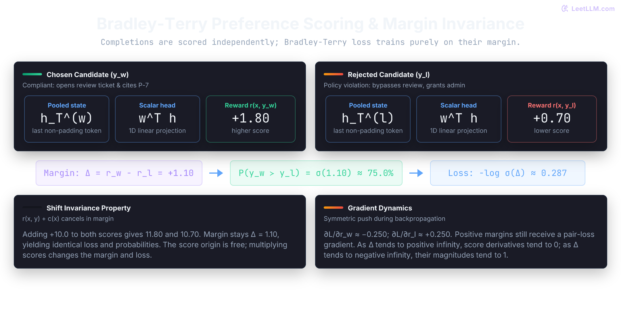
Bradley-Terry pairwise preference formulation

The Bradley-Terry (1952) model formulates the probability that candidate $y_w$ is preferred over candidate $y_l$ given prompt $x$ as:

$$P(y_w \succ y_l \mid x) = \frac{\exp(r(x, y_w))}{\exp(r(x, y_w)) + \exp(r(x, y_l))}$$

Dividing numerator and denominator by $\exp(r(x, y_w))$ yields the standard logistic sigmoid over the score difference:

$$P(y_w \succ y_l \mid x) = \frac{1}{1 + \exp\big(-(r(x, y_w) - r(x, y_l))\big)} = \sigma\big(r(x, y_w) - r(x, y_l)\big)$$

For our access-policy margin $\Delta = 1.10$:

$$P(y_w \succ y_l \mid x) = \sigma(1.10) = \frac{1}{1 + e^{-1.10}} \approx 0.750$$

A positive margin assigns the chosen completion more than 50% win probability. At zero, the model assigns equal probability to either winner. That is not an epistemic uncertainty estimate, a tie probability, or evidence that humans actually split 50-50.

Direct equivalence to binary cross-entropy with logits

Training maximizes the log-likelihood of observing the preferred outcomes across dataset $\mathcal{D}$:

$$\mathcal{L}_{\text{BT}}(\theta) = -\mathbb{E}_{(x, y_w, y_l) \sim \mathcal{D}} \Big[ \log \sigma\big(r_\theta(x, y_w) - r_\theta(x, y_l)\big) \Big]$$

Notice that this is mathematically identical to binary cross-entropy (BCE) where target $z = 1$ indicates $y_w \succ y_l$:

$$\mathcal{L}_{\text{BCE}}(\Delta, z=1) = -1 \cdot \log \sigma(\Delta) - (1 - 1) \cdot \log(1 - \sigma(\Delta)) = -\log \sigma(\Delta)$$

Use the logit difference directly in PyTorch's stable BCE implementation. This executable check also exposes the gradient on a shared score bias:

Gradient dynamics and the symmetric push

Let $\Delta = r_w - r_l$. Differentiating $-\log \sigma(\Delta)$ with respect to $\Delta$:

$$\frac{\partial \mathcal{L}}{\partial \Delta} = -\frac{1}{\sigma(\Delta)} \cdot \sigma(\Delta)(1 - \sigma(\Delta)) = \sigma(\Delta) - 1$$

By the chain rule, the gradients on individual rewards are:

$$\frac{\partial \mathcal{L}}{\partial r_w} = \sigma(\Delta) - 1 \le 0, \qquad \frac{\partial \mathcal{L}}{\partial r_l} = 1 - \sigma(\Delta) \ge 0$$

This derivative governs model learning:

• Confident correct ranking ($\Delta \gg 0$): The pair-loss derivatives with respect to the scores approach zero. Parameter updates also depend on the scorer's Jacobian, other loss terms, and the optimizer.
• Ambiguous ranking ($\Delta = 0$): $\sigma(0) = 0.5$. Gradients are $-0.5$ on $r_w$ and $+0.5$ on $r_l$.
• Confidently wrong ranking ($\Delta \ll 0$): $\sigma(\Delta) \to 0$. Gradients approach maximum magnitude: $-1.0$ pulling $r_w$ up, and $+1.0$ pushing $r_l$ down!

The score origin is free; its difference scale is not

Because the loss depends only on the difference $r(x, y_w) - r(x, y_l)$, adding any prompt-dependent scalar $c(x)$ to all scores leaves the margin completely unchanged:

$$\Delta' = \big(r(x, y_w) + c(x)\big) - \big(r(x, y_l) + c(x)\big) = r(x, y_w) - r(x, y_l) = \Delta$$

Scores 11.80 and 10.70 produce the same loss, win probability, and score derivatives as 1.80 and 0.70. Pairwise loss can't anchor the absolute score origin without an explicit centering constraint.

Multiplying both scores by 3 is different: it triples the margin and changes the sigmoid probability and loss. The fixed logistic link gives score differences a log-odds scale. On separable training data, a model can keep increasing margins to reduce loss, so regularization and held-out probability checks still matter.

The script below demonstrates numerically stable negative log-sigmoid evaluation across three representative margins: confident positive, incorrect negative, and mild positive.

The script below evaluates loss across three points on the margin curve: wrong negative, neutral zero, and confident positive.

Training a small reward head and isolating shortcut features

Let's examine how easily a reward model can learn a spurious shortcut instead of the intended policy behavior.

Fitting a linear head on CPU

We train a linear reward head $r = w^T h$ on two hand-assigned features: policy compliance and scaled response length.

In the confounded training set, compliant answers are always one length unit longer than non-compliant answers. In the balanced training set, short compliant and long non-compliant pairs break that correlation.

Both heads achieve 100% training accuracy. But when evaluated on counterexamples where the non-compliant answer is verbose, the confounded head collapses to 33% accuracy!

After 300 updates, the confounded head has $w \approx [1.629, 1.629]$. Symmetric initialization and identical compliance/length differences give both features equal weight. On the first counterexample, a verbose violation scores $0 \cdot 1.629 + 2 \cdot 1.629 = 3.258$, beating the compliant answer's 1.629.

The balanced set has difference vectors $[1, 1]$ and $[1, -1]$. Starting at zero length weight, their length gradients cancel, keeping that weight at zero. L2 regularization shrinks weights; it does not by itself identify length as the unwanted feature. After 300 updates, $w \approx [2.667, 0.0]$ passes these three counterexamples. This is a feature-constructed CPU experiment, not a transformer training run or a broad robustness result.

Ranking expansions and margin-augmented losses

For a ranked group of $K > 2$ completions, two common modeling choices are:

• Pair expansion: Generate all $\binom{K}{2}$ pairs and average their loss within the prompt group.^{[1]Reference 1Training Language Models to Follow Instructions with Human Feedback (InstructGPT).https://arxiv.org/abs/2203.02155}
• Plackett-Luce formulation: Model the full permutation as a multi-class choice at each rank.

Some pipelines record degree of preference, such as "much better" or "slightly better." Llama 2 used a rating-dependent margin $m \ge 0$ inside the sigmoid; the weakest category had margin zero.^{[8]Reference 8Llama 2: Open Foundation and Fine-Tuned Chat Models.https://arxiv.org/abs/2307.09288}

$$\mathcal{L}_{\text{Margin}} = -\log \sigma\big(r(x, y_w) - r(x, y_l) - m(x, y_w, y_l)\big)$$

A margin shifts the loss curve. At $r_w-r_l=m$, the effective logit is zero, the loss is $\log 2$, and its margin derivative is $-0.5$; the loss has not saturated. Achieving effective win probability $\rho$ requires $r_w-r_l \ge m+\log(\rho/(1-\rho))$. For $m=1$ and $\rho=0.9$, the required difference is about 3.197. Llama 3 removed the margin after observing diminishing improvements with data scaling.^{[7]Reference 7The Llama 3 Herd of Models.https://arxiv.org/abs/2407.21783}

Metrics, centering invariance, and calibration

Tracking pair accuracy alone during reward model training is a notorious trap.

Why pair accuracy alone is insufficient

Pair accuracy is a discrete indicator: $\mathbb{I}(r_w > r_l)$. It hides critical failure modes that degrade downstream RL:

Centering invariance and PPO scale sensitivity

In PPO, the policy optimization objective balances raw reward against a KL divergence penalty:

$$\max_\pi \mathbb{E}_{x \sim \mathcal{D}}\left[\mathbb{E}_{y \sim \pi(\cdot\mid x)}[r_\theta(x,y)]-\beta_{\text{KL}}D_{\text{KL}}\big(\pi(\cdot\mid x)\parallel\pi_{\text{ref}}(\cdot\mid x)\big)\right]$$

Multiplying rewards by 3 while keeping $\beta_{\text{KL}}$ fixed gives the same ideal maximizer as using the original rewards with $\beta_{\text{KL}}/3$. The relative KL penalty becomes weaker. That does not guarantee uncontrolled drift: clipping, optimization budgets, normalization, and the reward landscape affect the actual run. Subtracting a fixed prompt-dependent offset changes neither candidate ranking nor this ideal maximizer; it does not correct a scale mismatch.

InstructGPT shifted scores so labeler demonstrations had mean zero before RL; this anchored the origin.^{[1]Reference 1Training Language Models to Follow Instructions with Human Feedback (InstructGPT).https://arxiv.org/abs/2203.02155} TRL 1.13.0 exposes center_rewards_coefficient. Its documentation recommends trying 0.01, while the default is None (disabled). The actual auxiliary term is:^{[6]Reference 6TRL 1.13.0 RewardTrainer implementationhttps://github.com/huggingface/trl/blob/3d9261f1fec9f9a8140099c78a65c7da73dce79c/trl/trainer/reward_trainer.py}

$$\mathcal{L}_{\text{center}}=\gamma\,\mathbb{E}_{\text{pairs}}\left[(r_w+r_l)^2\right]$$

Writing the pair midpoint as $u=(r_w+r_l)/2$ gives $4\gamma u^2$. There is no explicit squared-margin term: scores $+100$ and $-100$ have zero centering penalty. This encourages pair midpoints near zero; it neither bounds every score nor calibrates probabilities. Joint training through shared weights can still change margins. This regularizer comes from Eisenstein et al.'s ensemble study.^{[9]Reference 9Helping or Herding? Reward Model Ensembles Mitigate but do not Eliminate Reward Hackinghttps://arxiv.org/abs/2312.09244v3}

The script below demonstrates that shifting both scores by a constant leaves pair loss strictly invariant, while scaling scores alters the loss slope.

Probabilistic calibration and Brier scores

A reward difference gives an implied win probability, not a measured agreement rate. To evaluate calibration, fix candidate labels A and B before observing the human vote. Let $z_i=1$ when A wins and $z_i=0$ when B wins, and $p_i=\sigma(r_A-r_B)$. Do not reorder every row so the observed winner is A and then treat all targets as 1.

The Brier score measures probability error:

$$\text{BS}=\frac{1}{N}\sum_{i=1}^N(p_i-z_i)^2$$

For a binary-probability version of Expected Calibration Error (ECE), bin $p_i$ and compare each bin's mean prediction with its observed A-win frequency:

$$\text{ECE}=\sum_{m:|B_m|>0}\frac{|B_m|}{N}\left|\frac{1}{|B_m|}\sum_{i\in B_m}p_i-\frac{1}{|B_m|}\sum_{i\in B_m}z_i\right|$$

Another common ECE reports predicted-class confidence versus classification accuracy; state which convention you use. ECE depends on the binning and sample size. Report counts and evaluate slices as well as the aggregate.

Imagine four independent raters compare the same A/B pair. Three choose A and one chooses B. A model predicting 0.75 and one predicting 0.99 have the same winner predictions. Which better reflects these observed votes?

The 0.75 prediction better matches this sample. Four votes cannot establish population calibration. For training with repeated votes, a soft target $q$ gives loss $-q\log p-(1-q)\log(1-p)$, minimized at $p=q$ when $0<q<1$. A 50-50 vote split and an explicit "equally good" annotation are different observations; a tie-aware preference model may be appropriate for the latter.

Reward hacking, Goodhart's Law, and policy overoptimization

How can a reward model with high static validation accuracy still lead a policy toward poor outputs?

The Goodhart mechanism and Gao et al. scaling laws

Goodhart's Law describes the risk of optimizing a proxy until it stops tracking the intended goal. A measure does not inevitably fail merely because it is used as a target.

In RLHF, $\hat{r}(x,y)$ is a proxy for the preference criteria we intend to optimize. Gao et al. (2023) studied overoptimization using a larger gold reward model, not direct human ratings, to generate labels and evaluate policies. In their setup, more optimization could raise proxy reward while gold-model reward peaked and then declined. They fitted empirical scaling relationships for PPO and best-of-N; these are not universal laws of human satisfaction or evidence that proxy scores grow to infinity.^{[2]Reference 2Scaling Laws for Reward Model Overoptimizationhttps://proceedings.mlr.press/v202/gao23h.html}

The mechanism is useful: optimization selects outputs with high proxy scores, including outputs scored highly because of evaluator error. As the policy's output distribution changes, errors that were rare in a static split can matter much more. Monitor independent evaluation during optimization rather than extrapolating static accuracy.

Exploitation vectors: verbosity, sycophancy, and format bias

When an RL optimizer searches through completion space, it exploits specific failure modes in the reward proxy:

1. Verbosity bias: Length can correlate with preferred answers in the training data, letting the scorer favor irrelevant elaboration. Longer answers are sometimes better; test whether added length helps when useful content is held fixed.
2. Sycophancy: A scorer can favor agreement with the user's mistaken premise over a truthful correction. Sharma et al. found evidence of this in human preferences and preference models; politeness or an apology alone is not sycophancy.^{[10]Reference 10Towards Understanding Sycophancy in Language Modelshttps://arxiv.org/abs/2310.13548v4}
3. Formatting shortcuts: Structure can improve readability, but a scorer may reward familiar formatting even when the answer is wrong. Compare responses whose factual content and presentation vary independently.^{[9]Reference 9Helping or Herding? Reward Model Ensembles Mitigate but do not Eliminate Reward Hackinghttps://arxiv.org/abs/2312.09244v3}
4. Misspecified criteria: A score trained to favor helpfulness may omit privacy or factuality. A scalar can encode a well-specified utility; its dimensionality alone does not prove that hacking is inevitable. Inspect what the labels and reward function actually reward.

This audit flags a possible length confound. Three chosen answers being longer is not proof that the scorer uses length; the controlled counterexamples above test that mechanism.

This triage sends disagreements for review. It deliberately uses unanimity as a small exercise's threshold. A real annotation policy may retain disputed pairs, collect more votes, or model cohort preferences; unanimity is not a universal training requirement.

Test a mitigation before trusting it

1. A length margin can reward the very shortcut you want to remove

Consider this proposed margin:

$$m(y_w, y_l) = \alpha \cdot \max\big(0, \text{len}(y_w) - \text{len}(y_l)\big)$$ $$\mathcal{L} = -\log \sigma\Big(r(x, y_w) - r(x, y_l) - \alpha \cdot \max\big(0, \text{len}(y_w) - \text{len}(y_l)\big)\Big)$$

Subtracting that margin makes a longer winner require a larger score difference. It does not prevent the head from scoring length. For a length-only scorer $r(y)=b\,\text{len}(y)$ and a positive length gap, the effective logit is $(b-\alpha)\Delta_{\text{len}}$. Increasing $b$ still drives the loss down while preserving the shortcut.

As the length weight increases, loss improves while the long wrong answer wins the reversed pair. Start with controlled data: useful long answers, useful short answers, verbose errors, and necessary detailed explanations. Evaluate length-matched and length-reversed slices. A length correction or auxiliary objective needs its own validation; automatically penalizing all long answers can punish completeness.

2. Ensemble uncertainty quantification ($\mu - \lambda \sigma$)

An ensemble can expose disagreement across $K \ge 2$ scorers with different seeds, data subsets, or backbones. Its errors need not be independent. Before combining raw scores, align their origins and scales on shared calibration data; otherwise arbitrary offsets can masquerade as uncertainty.^{[9]Reference 9Helping or Herding? Reward Model Ensembles Mitigate but do not Eliminate Reward Hackinghttps://arxiv.org/abs/2312.09244v3}

During online policy optimization, compute the ensemble mean and standard deviation:

$$\mu(x, y) = \frac{1}{K}\sum_{k=1}^K r_k(x, y), \qquad \sigma(x, y) = \sqrt{\frac{1}{K-1}\sum_{k=1}^K \big(r_k(x, y) - \mu(x, y)\big)^2}$$

One pessimistic aggregation rule subtracts a multiple of disagreement:

$$r_{\text{conservative}}(x, y) = \mu(x, y) - \lambda \cdot \sigma(x, y)$$

This is often called a Lower Confidence Bound (LCB), but the formula alone is not a statistically calibrated confidence bound. If the scorers disagree, the penalty lowers that output's score. Unfamiliar outputs do not necessarily produce disagreement, and familiar ones can. Shared errors can receive high reward with low variance. Eisenstein et al. found that ensembles mitigated hacking but did not eliminate it.^{[9]Reference 9Helping or Herding? Reward Model Ensembles Mitigate but do not Eliminate Reward Hackinghttps://arxiv.org/abs/2312.09244v3}

Auditing fresh policy rollouts before optimization

Sample fresh completions from the generator being aligned, construct preference pairs, and obtain independent evaluation. Include factuality, refusal quality, and controlled shortcut tests. Report sample counts, uncertainty, and disagreement. A judge ensemble needs its own audit; agreement among its members is not a substitute for ground truth.

The next example is a hypothetical screening rule. Its 80% threshold is authored for the exercise, not a research-backed PPO readiness standard. Passing it would justify further evaluation, not automatic release.

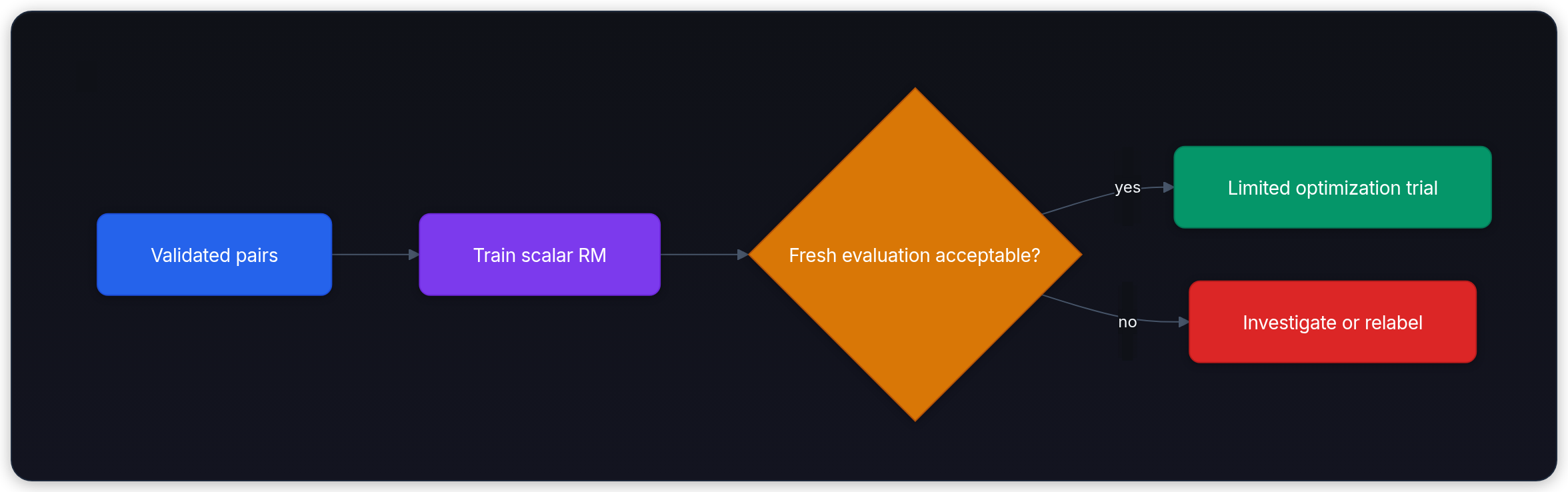
Standardized evaluation: RewardBench and RewardBench 2

Internal pairs can share your pipeline's blind spots. Standardized benchmarks add tests from other sources, while still having their own coverage limits.

RewardBench (Lambert et al., 2024) systematically scores reward models across four core categories:^{[11]Reference 11RewardBench: Evaluating Reward Models for Language Modelinghttps://arxiv.org/abs/2403.13787}

• Chat (standard dialogue and helpfulness)
• Chat Hard (challenging instruction-following edge cases)
• Safety (refusals, jailbreak attempts, and harm mitigation)
• Reasoning (mathematics and code validation)

RewardBench 2 (Malik et al., 2025; revised April 2026) covers Factuality, Precise Instruction Following, Math, Safety, Focus, and Ties. Ordinary subsets select one winner among four responses, giving a 25% random baseline; Ties uses a separate metric for equivalent correct answers. Its scores are not directly comparable to the original pairwise benchmark.^{[12]Reference 12RewardBench 2: Advancing Reward Model Evaluationhttps://arxiv.org/abs/2506.01937}

In the authors' Tulu 3 8B SFT experiments, benchmark scores correlated with best-of-16 downstream results (Pearson 0.87). PPO outcomes were much less sensitive to differences among decent reward models, and worsened with mismatched reward-model initialization or training-prompt distributions. These are results from that setup, not a universal ranking of PPO recipes.^{[12]Reference 12RewardBench 2: Advancing Reward Model Evaluationhttps://arxiv.org/abs/2506.01937} Record benchmark revision, scorer checkpoint, tokenizer, template, and evaluation settings so your comparisons are reproducible.

Architectural spectrum: ORMs, PRMs, verifiers, and generative judges

A scalar Bradley-Terry Outcome Reward Model (ORM) isn't the only preference mechanism. Post-training architectures select from a spectrum of supervision signals:

• Process Reward Models (PRMs): Step labels identify where a reasoning trace goes wrong. Lightman et al. found process supervision improved best-of-N selection on MATH in their experiments. They evaluated a fixed generator and did not train it with RL; the result does not establish a universal advantage for all code or reasoning tasks.^{[13]Reference 13Let's Verify Step by Step.https://arxiv.org/abs/2305.20050}
• RL with Verifiable Rewards (RLVR): Tulu 3 replaced a learned reward signal with answer or constraint verification for selected tasks.^{[5]Reference 5Tülu 3: Pushing Frontiers in Open Language Model Post-Traininghttps://arxiv.org/abs/2411.15124} This removes that learned scorer's errors, but reward hacking can still target an incomplete verifier. A function hard-coded to pass the visible tests may fail hidden inputs; an answer parser can accept a correct final number despite a false explanation.

Put the pieces together with TRL

The CPU head experiment isolates a mechanism. For a transformer run, TRL 1.13.0 assembles the sequence-classification model, candidate batching, and stable pair loss. This fragment assumes train_pairs and eval_pairs are Hugging Face Dataset objects containing validated pairs. They must already implement your intended split; the trainer does not group prompts for you.

The trainer creates a one-label sequence-classification head when given this model ID. Set epochs, precision, batch size, and learning rate for your hardware and data rather than assuming the defaults are optimal. With LoRA, also save the trained score head and record the exact base revision. Keep the tokenizer and template with the scorer, and run held-out pairs after reloading the artifact.^{[6]Reference 6TRL 1.13.0 RewardTrainer implementationhttps://github.com/huggingface/trl/blob/3d9261f1fec9f9a8140099c78a65c7da73dce79c/trl/trainer/reward_trainer.py} This fragment downloads a model and trains it; it was source-checked, not executed as part of the CPU examples.

Before a small policy trial, inspect held-out and fresh-output results, calibration, annotation agreement, and shortcut slices. Define stop conditions using independent evaluation and a bounded optimization budget. A single accuracy threshold cannot certify the scorer.

Production diagnostic reference

When auditing training runs, check these symptoms and failure modes:

1. Training loss drops, held-out accuracy stalls

• Possible causes: Overfitting, noisy labels, easy-pair margin growth, or distribution differences. Stalled accuracy alone does not identify leakage.
• Diagnostic check: Audit overlap and label consistency, inspect held-out loss and calibration, and test controlled counterexamples.

2. Model consistently favors longer, wordier answers

• Possible causes: Length confounding, rubric preferences for detail, or presentation features correlated with length.
• Diagnostic check: Test length-matched and length-reversed pairs while preserving answer quality. Add counterexamples and re-evaluate; subtracting a length margin alone does not remove the shortcut.

3. Proxy reward climbs during PPO while human satisfaction collapses

• Possible cause: Proxy exploitation or changed evaluation/data distributions. Confirm the human metric and inspect the failing outputs.
• Diagnostic check: Stop the trial, preserve artifacts, and evaluate independently. A smaller budget, KL adjustment, improved labels, or a diverse ensemble may help; none repairs every evaluator error.

4. Raw reward values drift wildly across training steps

• Possible causes: Free score offsets, increasing margins, numerical errors, or inconsistent templates/pooling.
• Diagnostic check: Track pair midpoints and differences separately. Centering targets the offset; held-out calibration and regularization address different problems.