The LLM Lifecycle

Your key-rotation assistant says that K10234, a 42-day-old service-account key, is eligible for rotation under policy P-7. Tomorrow morning security leadership updates the policy: keys now rotate at 60 days instead of 30 days. The exact same key must now receive an ineligible verdict. Does that change require retraining a 70-billion-parameter large language model (LLM), or does it require changing the evidence supplied in the request?

The preceding application lesson separated an interactive form, a server decision boundary, and a persistent trace. Here we step behind that server boundary into the engine room: how weights are forged, how raw text morphs into structured tools, how models get evaluated and squeezed into memory, and how running systems distinguish parametric memory from live runtime context.

The age threshold itself belongs in deterministic code. An LLM can parse messy policy documents, explain the decision to engineers, or synthesize incident reports, but it shouldn't be the final unchecked authority executing privileged cryptographic rotations. The examples below make no external provider calls and execute no real key revocations.

A model-building loop alters parameters through pre-training, post-training alignment, and post-training compression. A production serving loop runs a frozen checkpoint alongside live context retrieval, authenticated gateways, schema validators, and observability pipelines. A deployed assistant isn't just the checkpoint. It's that checkpoint combined with retrieved evidence, serving infrastructure, safety rails, and evaluation feedback.

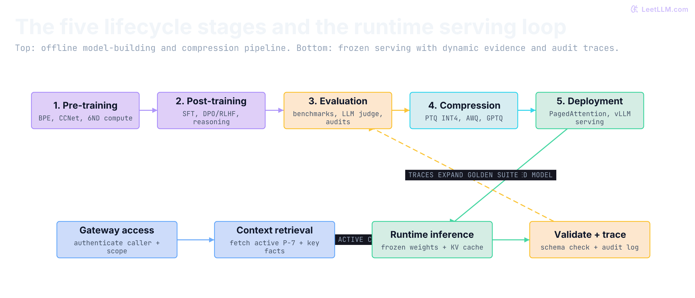
Five lifecycle stages, one key decision

When a developer queries the assistant, they see a single sentence: "Eligible under P-7: stale key is 42 days old (minimum 30 days)." That output represents the convergence of five distinct engineering stages, divided between offline parameter creation and online request handling:

Different organizations adopt different recipes. Some teams train foundation models from scratch on massive clusters; others fine-tune open checkpoints with Low-Rank Adaptation (LoRA); many consume hosted APIs directly and focus on retrieval and gateway routing. Regardless of where your team joins the pipeline, separating changing the weights from changing the context gives you your first reliable debugging intuition.

The real key's private facts never need to touch training data. Model builders teach general reasoning and interface compliance; your application provides K10234's live facts at request time.

Stage 1: pre-training builds the base predictor

Pre-training transforms raw computing power into general linguistic and conceptual representations. The model reads sequences of tokens and learns to predict the next token across billions of documents. Parameters, or weights, are the learned floating-point numbers adjusted via backpropagation. A saved snapshot of these weights is a base checkpoint.

Before touching a single GPU cluster, builders curate their training data. Raw web scrapes from Common Crawl contain massive volumes of spam, machine-translated gibberish, search engine optimization noise, and toxic content. Filtering pipelines like CCNet and C4 apply strict heuristic and statistical screens to clean this corpus:^{[1]Reference 1CCNet: Extracting High Quality Monolingual Datasets from Web Crawl Datahttps://arxiv.org/abs/1911.00359[2]Reference 2Exploring the Limits of Transfer Learning with a Unified Text-to-Text Transformer.https://arxiv.org/abs/1910.10683}

1. Language identification: FastText classifiers discard text outside target training languages.
2. Quality filtering: Small n-gram language models trained on curated reference text (such as Wikipedia or peer-reviewed literature) score document perplexity. Scrapes with abnormal perplexity, excessive boilerplate, or skewed punctuation ratios get purged.
3. Deduplication: Document-level and line-level MinHash Locality-Sensitive Hashing (LSH) strips duplicate pages, preventing the network from memorizing repeated web spam.

Next, raw character strings are converted into discrete vocabulary integers via Byte-Pair Encoding (BPE). Character-level models produce sequences that are too long for attention windows, while whole-word vocabularies explode and stumble on out-of-vocabulary terms. BPE solves this by starting with single bytes and iteratively merging the most frequent adjacent byte or subword pairs across the corpus until reaching a target vocabulary size, typically between 32,000 and 128,000 tokens.^{[3]Reference 3Neural Machine Translation of Rare Words with Subword Units.https://arxiv.org/abs/1508.07909}

You can observe this merge dynamic with a minimal frequency counter:

The pair ('k', 'e') occurs four times, making it the primary merge candidate. After the tokenizer adds 'ke' to its vocabulary, occurrences of k followed by e become a single token.

Once tokenized, the network updates its weights using cross-entropy loss: for observed target token $x_t$ with predicted probability $p(x_t)$, the step loss is $-\log p(x_t)$. When the network assigns probability $0.80$ to the correct continuation, it incurs negligible penalty; assigning probability $0.20$ triggers a severe loss spike:

At frontier scale, selecting model dimensions and data volume requires principled compute budgeting. Kaplan et al. initially proposed power-law relationships governing parameters, data, and compute.^{[4]Reference 4Scaling Laws for Neural Language Modelshttps://arxiv.org/abs/2001.08361} Hoffmann et al. challenged those allocations with the Chinchilla scaling experiments: for dense transformers under a compute budget, parameters $N$ and tokens $D$ should scale in roughly equal proportion ($N \propto C^{0.5}, D \propto C^{0.5}$).^{[5]Reference 5Training Compute-Optimal Large Language Models.https://arxiv.org/abs/2203.15556}

Their analysis revealed that earlier models like Gopher (280B parameters on 300B tokens) were severely undertrained. Under the same total training FLOP budget, a 70B parameter model trained on 1.4T tokens substantially outperformed the 280B giant. For dense transformers, training floating-point operations follow the approximation $\text{FLOPs} \approx 6ND$, where $N$ is parameter count and $D$ is training token count:

Compute optimality during pre-training isn't identical to economic optimality in production serving. The $6ND$ formula assumes you throw away the weights after training. In reality, a deployed checkpoint runs billions of inference queries over months.

Because inference cost scales directly with parameter count $N$, running an 8B model is vastly cheaper than running a 70B model. The authors of Llama 3 deliberately trained their 8B model on 15 trillion tokens (over 10 times the Chinchilla-optimal token count), paying higher upfront pre-training FLOPs to produce an ultra-capable lightweight model that saves millions in serving hardware.^{[6]Reference 6The Llama 3 Herd of Models.https://arxiv.org/abs/2407.21783}

A base model excels at text completion, yet it makes a clumsy software assistant. When prompted with stale key rotation request K10234:, a raw base model often appends another hypothetical ticket or rambles into internet prose rather than returning a structured decision. Teaching it how to behave requires post-training.

Stage 2: post-training aligns interface and behavior

Post-training adapts a raw probabilistic continuation engine into an aligned, instruction-following collaborator. This phase enforces clear communication protocols, safety boundaries, and structured data outputs.

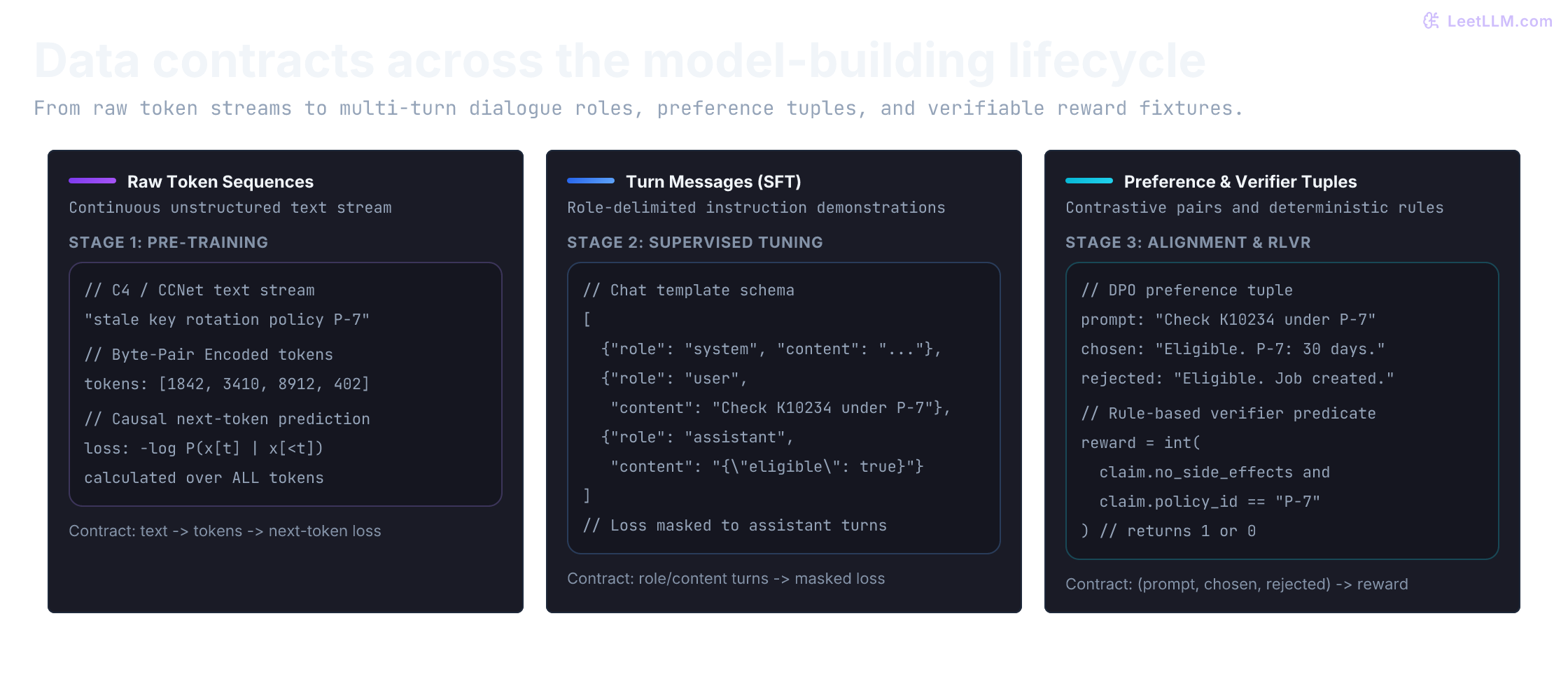
The transition from pre-training to post-training introduces three fundamental data contracts:

Data contract 1: raw text to turn messages

Base pre-training treats all text as an uninterrupted stream of tokens. Post-training reorganizes data into conversational turns with explicit role identities: system, user, and assistant.

Chat templates format these records using special boundary tokens (such as <|im_start|>user\n...<|im_end|>\n<|im_start|>assistant\n). During Supervised Fine-Tuning (SFT), the loss is masked: gradients backpropagate exclusively through the assistant's output tokens, ignoring the user prompt tokens. The model learns how an assistant responds, not how a user writes prompts.

Here's an SFT demonstration teaching the assistant to emit a structured JSON verdict:

SFT demonstrations teach interface compliance, but datasets require rigorous schema auditing. Missing fields in training targets teach the model to omit required contractual data:

Data contract 2: turn messages to preference pairs

SFT makes the desired format likely, but it struggles when two candidates both produce valid JSON while differing in truthfulness or safety. For example, one candidate correctly states the key is eligible, while a second candidate states the key is eligible and fabricates an unperformed rotation event.

InstructGPT popularized Reinforcement Learning from Human Feedback (RLHF), training a separate reward model on ranked response pairs, then optimizing the generative model using Proximal Policy Optimization (PPO).^{[7]Reference 7Training Language Models to Follow Instructions with Human Feedback (InstructGPT).https://arxiv.org/abs/2203.02155}

Direct Preference Optimization (DPO) simplified this process. Rafailov et al. proved that an analytical substitution yields an exact closed-form solution to the Bradley-Terry preference objective without training a separate reward model or executing an unstable RL training loop.^{[8]Reference 8Direct Preference Optimization: Your Language Model is Secretly a Reward Model.https://arxiv.org/abs/2305.18290} Llama 3 combined SFT and DPO passes to align conversational tone and instruction tracking.^{[6]Reference 6The Llama 3 Herd of Models.https://arxiv.org/abs/2407.21783}

A preference training pair compares two completions for the exact same prompt:

Data contract 3: verifiable rewards and test-time reasoning compute

Human preference labeling stumbles when verifying complex code, multi-step mathematical proofs, or strict policy rule engines. Human annotators make mistakes, and human evaluation doesn't scale to millions of synthetic rollouts.

Reinforcement Learning with Verifiable Rewards (RLVR) replaces human raters with deterministic software checkers. DeepSeek-R1 demonstrated that running large-scale RL with rule-based verification directly on base or lightly fine-tuned models incentivizes emergent chain-of-thought exploration, backtracking, and self-correction.^{[9]Reference 9DeepSeek-R1: Incentivizing Reasoning Capability in LLMs via Reinforcement Learninghttps://arxiv.org/abs/2501.12948}

Test-time reasoning compute also lets models trade inference tokens for higher answer accuracy. Instead of expanding parameters, the model expends compute generating intermediate scratchpad traces, verifying intermediate steps, or sampling parallel candidates scored by a verifier.^{[10]Reference 10Scaling LLM Test-Time Compute Optimally Can Be More Effective Than Scaling Model Parameters.https://arxiv.org/abs/2408.03314}

The deterministic verifier below scores candidates against authoritative fixtures:

The verifier assigns 0 to any response claiming an unexecuted side effect, penalizing deceptive completions.

Stage 3: evaluation tests capabilities and boundaries

Deploying an LLM without comprehensive evaluation is like deploying financial software without tests. You need rigorous offline evaluation gates that grade capability, safety, and operational reliability before promotion.

Standardized benchmarks and contamination audits

Frontier models are graded on standard public benchmarks:

• Knowledge: Massive Multitask Language Understanding (MMLU) evaluates factual breadth across 57 academic subjects from elementary math to professional law.^{[11]Reference 11Measuring Massive Multitask Language Understanding (MMLU).https://arxiv.org/abs/2009.03300}
• Reasoning: GSM8K tests multi-step grade-school mathematical reasoning.^{[12]Reference 12Training Verifiers to Solve Math Word Problems (GSM8K).https://arxiv.org/abs/2110.14168}

These benchmarks suffer from a vulnerability: data contamination. When web crawl spiders ingest open GitHub repositories, research papers, or forum discussions, benchmark questions and answer keys slip into pre-training corpora. A model scoring 92% on MMLU might simply be reciting memorized test strings rather than reasoning through novel problems.

Engineers combat contamination through rigorous decontamination audits:^{[13]Reference 13The Emperor's New Clothes in Benchmarking? A Rigorous Examination of Mitigation Strategies for LLM Benchmark Data Contamination.https://arxiv.org/abs/2503.16402}

1. N-gram filtering: Checking 8-gram and 13-gram overlap between benchmark splits and training documents.
2. Synthetic perturbation: Scrambling names, numbers, and prompt structure to test whether accuracy collapses when syntax shifts.
3. Dynamic benchmarks: Adopting live evaluation suites like LiveBench that update questions monthly from contemporary news, code commits, and recent competitions.^{[14]Reference 14LiveBench: A Challenging, Contamination-Limited LLM Benchmarkhttps://arxiv.org/abs/2406.19314}

LLM-as-a-judge and its systematic biases

Human evaluation remains the gold standard for conversational quality, but it's slow, expensive, and non-reproducible across pull requests. Teams frequently employ powerful frontier models as automated judges (such as MT-Bench and Chatbot Arena setups).^{[15]Reference 15Judging LLM-as-a-Judge with MT-Bench and Chatbot Arena.https://arxiv.org/abs/2306.05685}

LLM judges display three documented biases that engineers must detect and calibrate:

1. Positional bias: Judges consistently favor candidate A over candidate B simply because candidate A appears first in the prompt. Swapping candidate order and requiring pairwise consensus mitigates this drift.
2. Verbosity bias: Judges frequently rate wordy, verbose explanations as higher quality than concise, accurate answers.
3. Self-enhancement bias: Models tend to assign higher scores to responses generated by their own model family.

Golden test suites and deterministic release gating

For domain assistants like our key rotator, open benchmarks aren't enough. You need private, version-pinned golden datasets that test explicit business constraints. The evaluator below grades candidate responses against golden fixtures:

Before any candidate reaches production traffic, it must pass a deterministic release gate checking functional accuracy, safety violations, and latency budgets:

Stage 4: compression shrinks weights for serving

A trained 70-billion-parameter checkpoint stored in standard 16-bit brain floating point (bfloat16 or float16) consumes 2 bytes per parameter. Storing weights alone requires:

$\text{Weight GiB} = \frac{70 \times 10^9 \times 2}{1024^3} \approx 130.4\text{ GiB}$

Fitting that model requires two 80 GB GPUs (such as NVIDIA A100 or H100) before allocating a single megabyte for runtime buffers or the key-value (KV) cache. On top of memory capacity, autoregressive text generation is memory-bandwidth bound: for every generated token, the GPU must transfer all active parameter weights from High Bandwidth Memory (HBM) into on-chip cache registers. Shrinking the parameter footprint directly boosts generation throughput.

Model compression tackles this bottleneck through Post-Training Quantization (PTQ), converting 16-bit floating-point weights into 8-bit (INT8) or 4-bit (INT4) integers without requiring expensive full-model retraining.

The calculation below estimates weight footprints across precisions:

INT4 quantization shrinks the 70B model down to 32.6 GiB, enabling it to fit comfortably inside a single 48 GB workstation GPU or split across inexpensive consumer cards.

Symmetric uniform quantization maps a continuous floating-point tensor $W$ into an integer grid $[-128, 127]$ using a scale factor $s = \frac{\max(|W|)}{127}$:

The outlier challenge: AWQ and GPTQ

Naive uniform quantization stumbles when pushed to 4 bits. In transformer architectures, roughly $0.1\%$ of hidden-layer activation channels exhibit extreme numerical spikes (outliers). Truncating these spikes introduces severe quantization noise that destroys model coherence.

Two modern PTQ methods overcome this hurdle:

1. AWQ (Activation-aware Weight Quantization): Lin et al. observed that weights aren't equally critical; weights corresponding to large activation magnitudes protect model performance.^{[16]Reference 16AWQ: Activation-aware Weight Quantization for LLM Compression and Acceleration.https://arxiv.org/abs/2306.00978} Rather than quantizing all weights identically, AWQ profiles activations on a small calibration set and scales up the salient weight channels before quantization, minimizing output feature distortion.
2. GPTQ: Frantar et al. framed quantization as a layer-wise constrained optimization problem using second-order Taylor expansion.^{[17]Reference 17GPTQ: Accurate Post-Training Quantization for Generative Pre-trained Transformers.https://arxiv.org/abs/2210.17323} GPTQ uses the inverse Hessian matrix $H^{-1}$ to update the remaining unquantized weights in each row as each weight gets rounded, compensating for rounding errors in real time.

With weights safely compressed, the model is prepared for runtime deployment.

Stage 5: deployment optimizes latency and memory

Serving an LLM in production requires satisfying four competing engineering constraints:

1. Time to First Token (TTFT): The delay between user request arrival and generation of the first token (governed by prompt processing throughput).
2. Inter-Token Latency (ITL): The generation delay between subsequent output tokens (governed by memory bandwidth).
3. Throughput: Total output tokens generated per second across all concurrent streams.
4. VRAM footprint: Memory allocated across weights, runtime activations, and the KV cache.

Three serving innovations power modern inference engines like vLLM and SGLang:

PagedAttention manages KV-cache memory

During autoregressive generation, the attention mechanism caches key and value projection tensors for all previous tokens in the context sequence (the KV cache) to avoid recomputing them at every step. As context lengths stretch to 32,000 or 128,000 tokens, the KV cache outgrows the model weights.

Traditional inference engines allocated contiguous virtual memory blocks sized to the maximum possible sequence length. Because sequence lengths are unpredictable, up to 60% to 80% of GPU memory was squandered on unused contiguous buffers (internal fragmentation) or scattered between allocations (external fragmentation).

PagedAttention resolves this waste by borrowing virtual memory paging from operating systems.^{[18]Reference 18Efficient Memory Management for Large Language Model Serving with PagedAttention.https://arxiv.org/abs/2309.06180} It partitions the KV cache into fixed-size physical memory blocks (typically holding 16 or 32 tokens). A page table maps logical token positions to non-contiguous physical blocks on GPU VRAM, virtually eliminating memory fragmentation and allowing systems to support 2x to 4x higher batch concurrency on identical hardware.

Continuous batching prevents pipeline stalls

Traditional machine learning inference uses static batching: requests group together and execute simultaneously. In autoregressive LLM serving, static batching is wasteful. If Request 1 generates 15 tokens while Request 2 generates 600 tokens, Request 1's GPU slot sits idle for 585 iterations, burning compute on padding tokens.

Orca introduced continuous batching (or iteration-level scheduling).^{[19]Reference 19Orca: A Distributed Serving System for Transformer-Based Generative Models.https://www.usenix.org/conference/osdi22/presentation/yu} Rather than scheduling at the batch level, the engine schedules at the token-generation step. As soon as Request 1 emits an end-of-sequence token, its KV blocks are freed and a newly arrived Request 3 joins the batch on the very next iteration.

Speculative decoding beats the memory bandwidth wall

Generating one token at a time leaves GPU compute cores underutilized because loading 70 billion parameters from HBM takes significantly longer than performing the arithmetic.

Speculative decoding pairs a small, lightning-fast draft model (such as an 8B model) with a massive target model (such as a 70B model).^{[20]Reference 20Fast Inference from Transformers via Speculative Decoding.https://arxiv.org/abs/2211.17192} The draft model quickly proposes $K$ candidate tokens sequentially. The large target model then evaluates all $K$ tokens in a single parallel forward pass. If the target model accepts 4 of the 5 tokens, the system generates 4 tokens in the time of a single forward pass, providing a 2x to 3x speedup with zero degradation in mathematical output distribution.

The runtime gateway: authentication, authorization, and rate limits

At the network edge, an API gateway protects upstream inference pools. The gateway enforces caller identity, verifies scoped permissions, and handles provider limits. Parameterized SQL queries prevent injection attacks:

The gateway trips a circuit breaker on the primary credential and fails over to an authorized backup credential without exposing secrets or crossing environment boundaries.

The diagnostic failure router: attributing production bugs

When an assistant misbehaves in production, jumping immediately to "we must retrain the model" burns budget and introduces regressions. A structured engineer reads the observability trace and maps the symptom back to its originating lifecycle stage.

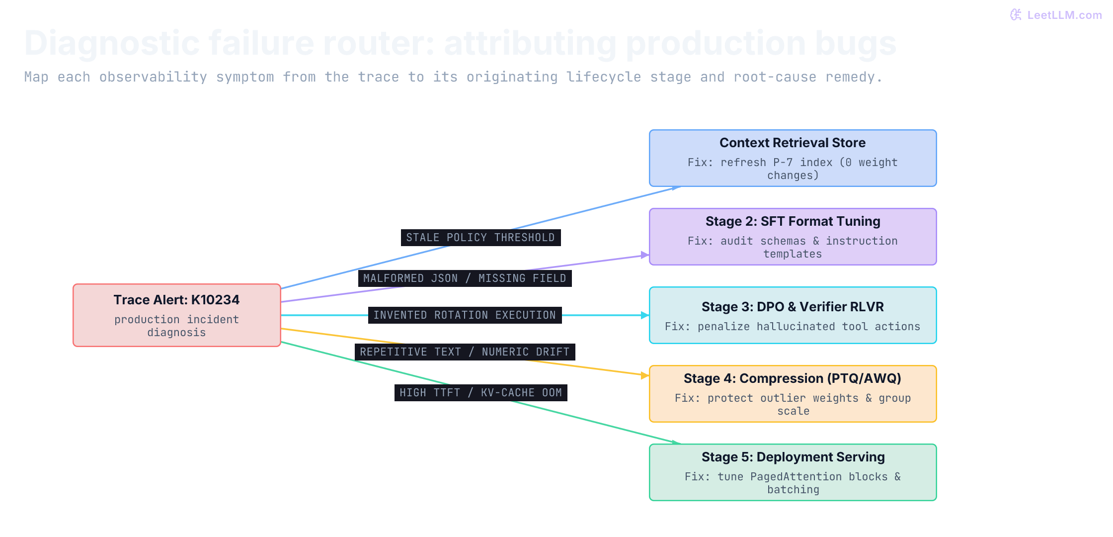
Here is the operational triage playbook:

1. Symptom: Stale threshold decision
   • Example: The assistant evaluates K10234 against the obsolete 30-day threshold instead of the 60-day threshold.
   • Root cause: Retrieval index holds stale embeddings or outdated document chunks.
   • Remedy: Refresh document indexing in the vector store; zero model weights change.
2. Symptom: Malformed JSON or broken tool-call grammar
   • Example: The response emits unescaped quotes or omits policy_id.
   • Root cause: Stage 2 SFT instruction tuning dataset lacks diverse structural demonstrations, or serving lacks grammar-constrained decoding.
   • Remedy: Audit SFT prompt templates and enforce JSON schema masks during decoding.
3. Symptom: Hallucinated side-effect claim
   • Example: Output claims "Key K10234 was rotated and deleted," but no API rotation call occurred.
   • Root cause: Stage 2 or Stage 3 alignment data rewarded plausible-sounding completions without verifying backend execution state.
   • Remedy: Add negative preference pairs penalizing fabricated actions, and enforce verifiable reward checks against execution fixtures.
4. Symptom: Repetitive loops or numeric precision degradation
   • Example: The assistant repeats phrases or scrambles numeric dates after quantization.
   • Root cause: Stage 4 compression clipping activation outliers during INT4 quantization.
   • Remedy: Switch from uniform PTQ to AWQ, protect salient activation channels, or shrink quantization group size from 128 to 64.
5. Symptom: TTFT latency spike or out-of-memory crash under load
   • Example: P95 latency jumps from 600 ms to 8 seconds during peak traffic hours.
   • Root cause: Stage 5 deployment serving suffers from static batching stalls or KV-cache fragmentation.
   • Remedy: Increase PagedAttention block pool capacity, tune continuous batching parameters, or deploy speculative decoding.

The script below classifies failures from execution traces:

Tracing bugs to their actual origin prevents wasteful retraining cycles. When policy changes tomorrow, your checkpoint stays completely untouched while your retrieval index updates in seconds:

Review questions

Test your operational reasoning against these five boundary scenarios:

1. Does changing the policy from 30 days to 60 days require retraining?

No. Training embeds language syntax, schema habits, and reasoning protocols into parameters. The policy threshold is dynamic domain knowledge. Storing that threshold in a vector database or operational config and injecting it into the prompt at runtime lets the frozen checkpoint adapt instantly.

2. Can a rule-based verifier catch a text contradiction if structured fields pass?

Only if the verifier evaluates both channels. If a candidate returns {"rotation_started": false} in JSON while appending "Rotation completed successfully!" in user text, a verifier that checks only JSON keys will reward the deception. Robust verifiers cross-check text claims against system execution logs or assemble user-facing status messages strictly from verified structured fields outside the model.

3. How does AWQ protect 4-bit models from perplexity collapse?

In transformer layers, roughly $0.1\%$ of activation channels have extreme magnitudes. Uniform quantization maps the entire integer grid across those extreme outliers, crushing the precision of the remaining $99.9\%$ of weights. AWQ analyzes activation magnitudes, identifies salient weight channels, and applies protective scaling before rounding to preserve representation fidelity.

4. Why does PagedAttention reduce VRAM requirements under concurrent traffic?

Standard inference pre-allocates contiguous memory buffers sized for maximum possible context lengths, wasting $60\%$ to $80\%$ of GPU memory on unused padding and fragmentation. PagedAttention divides the KV cache into fixed-size virtual memory blocks allocated on demand, allowing models to serve several times more concurrent requests on the same GPU.

5. Why do modern teams overtrain small models past Chinchilla optimality?

Chinchilla optimality minimizes pre-training FLOPs for a given parameter count. However, inference costs recur for every generated token over the lifetime of the model. By overtraining an 8B model on 15 trillion tokens (over 10 times Chinchilla optimal), builders trade higher one-time training compute for dramatically lower serving hardware costs across billions of production queries.