Personalize this lesson
Adapt explanations and teaching visuals to your background and preferred voice.
Continuous batching can refill decode slots as soon as a request finishes. A full queue can still hide a capacity failure: once the scheduler is willing to admit more work, what runs out first on the GPU serving a large language model (LLM)?
A code-assistant pool makes the constraint concrete. Short completions and long patch explanations share one model replica, and each request advances one token at a time during ordinary decode.
Each decode step reads model weights from GPU high-bandwidth memory (HBM) and consults a growing KV cache. For small-batch dense-model decode, moving those bytes often costs far more time than the arithmetic. Memory capacity separately limits how many concurrent streams fit in VRAM.
Start with an 8B-class replica on one GPU. As we add requests, its weights stay fixed but its KV occupancy grows. The larger 70B architecture stress-tests the same calculation. The CPU examples below check arithmetic, scheduling, and sampling behavior; they don't measure GPU throughput or run a live serving engine.
Why isn't "keep the batch full" enough to scale LLM serving?
Answer
A full batch still has to fit in HBM and still has to move weights plus KV state every decode step. If bandwidth or KV residency is the ceiling, extra admitted requests queue or stall instead of raising useful tokens per second.
Decode sits under a bandwidth roof
You already know the two phases from inference mechanics. Prefill reads known prompt tokens in parallel and is compute-heavy.
Decode emits one new token per request step. This sequential dependency is why a request can have prompt processing behind it but still need hundreds of serial iterations to finish.
Users wait for queueing, prompt processing, and delivery before the first token: together these make up time to first token (TTFT). During decode they experience inter-token latency (ITL), also called time between tokens (TBT). For a response with at least two tokens, time per output token (TPOT) averages the interval from first to last over the remaining tokens. A steady mean can easily mask a terrible p95 ITL.[1]
The root physical constraint is the split in arithmetic intensity. Arithmetic intensity measures FLOPs performed per byte loaded from HBM.
Prefill reuses each weight matrix across many prompt positions in matrix multiplications (GEMMs). One-request decode makes the dense linear operations matrix-vector products (GEMVs); batched decode uses thin GEMMs. Attention over cached history adds separate work.
For a dense model with parameters, use roughly FLOPs per token for the parameter-dependent linear work. This omits context-dependent attention and counts multiply-add as two FLOPs. If one step streams the weights once across batch size and weight reads dominate traffic, the simplified intensity is:
For FP16 precision (), the operational intensity simplifies to FLOPs per byte.
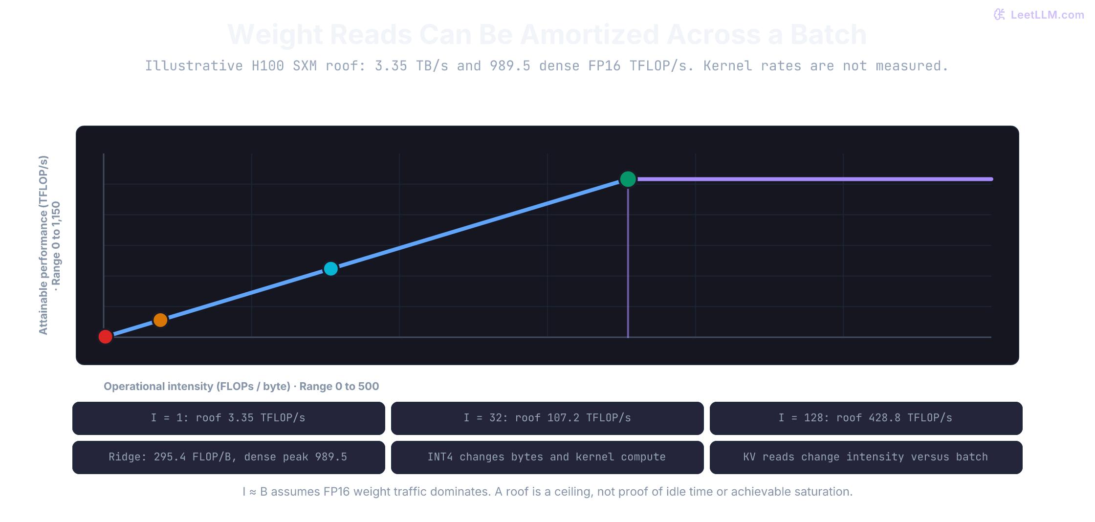
The roofline model bounds performance by the smaller of a compatible compute peak and memory bandwidth times intensity.[2][3] Below the ridge, the bandwidth roof is lower; above it, the compute roof is lower. Reaching either roof still requires suitable kernels and achieved hardware rates.
For H100 SXM, use peak HBM bandwidth of 3.35 TB/s and about 989.5 TFLOP/s of dense FP16/BF16 Tensor Core compute. NVIDIA's 1,979 figure includes sparsity and must be halved for this dense comparison.[4] The illustrative ridge is:
At , the weight-only approximation gives 1 FLOP/byte and a 3.35 TFLOP/s bandwidth roof, about 0.34% of that compute peak. This compares rates; it does not mean the tensor cores are idle for 99.66% of elapsed time. Device counters and a trace are needed to describe utilization.
Llama 3 8B is an 8B-parameter dense model.[5] An FP16 copy of those weights occupies about 16 GB (8e9 * 2 bytes).
If one uncached decode step streams that entire footprint for one active token, the weight-read upper bound on H100 SXM is 3350 / 16 ≈ 209 single-token steps per second. That's an idealized bandwidth thought experiment, not a promise about a production runtime.
Under that full-read assumption, dynamic KV cache traffic, attention calculations, and runtime overhead push the achievable rate lower. This isn't an unchangeable bound: weight quantization, speculative decoding, and batching all alter the equation. Use it as an immediate diagnosis: if a trace saturates HBM while tensor cores sit idle, buying more FLOPs won't speed up decode.
parameters = 8_000_000_000  # Llama 3 8B-class dense count
bytes_per_parameter = 2  # FP16
h100_sxm_hbm_gb_s = 3_350  # decimal GB/s, NVIDIA H100 SXM

weight_gb = parameters * bytes_per_parameter / 1_000_000_000
ideal_steps_per_second = h100_sxm_hbm_gb_s / weight_gb

print(f"FP16 weight footprint: {weight_gb:.1f} GB")
print(f"H100 SXM weight-read upper bound: {ideal_steps_per_second:.1f} single-token steps/s")
print("Under this full-read model, extra traffic and overhead can only lower the bound.")FP16 weight footprint: 16.0 GB
H100 SXM weight-read upper bound: 209.4 single-token steps/s
Under this full-read model, extra traffic and overhead can only lower the bound.You profile decode and see tensor cores idle while HBM bandwidth is near saturation. Should you first buy more FLOPs or reduce memory traffic?
Answer
Reduce bytes per emitted token or amortize them across a larger effective batch. Weight quantization targets weight reads; KV quantization targets cache reads and capacity. Paging improves allocation, not the payload bytes read. GQA/MQA requires choosing or adapting a checkpoint, not flipping an allocator flag.
KV bytes cap the batch you can form
Batching only helps if extra requests fit. The KV cache lesson derived the payload formula: each token stores a Key vector and a Value vector at every layer and KV head.
Llama 3 uses grouped-query attention with 8 KV heads at 8B, 70B, and 405B.[5][6] That head count is why KV state is much smaller than a full multi-head attention cache, but it still grows linearly with layers, sequence length, and concurrency.
For Llama 3 70B in FP16 (), one single token demands 2 * 80 * 8 * 128 * 2 = 327,680 bytes, or 320 KiB. Multiplying by 8,192 tokens yields 2.5 GiB per request. Sixty-four concurrent 8K streams require 160 GiB of KV cache alone, before loading a single weight byte. An 80 GB H100 can't hold that batch: a plan to keep cranking batch size until the roofline saturates crashes into VRAM residency first.
The smaller 8B model fits on a single accelerator. Llama 3 8B has 32 layers, 8 KV heads, and , requiring 128 KiB per token. A 4,096-token request takes exactly 0.5 GiB.[5]
For independent, unshared full-attention histories of the same length , a fixed pool gives a payload-only batch ceiling:
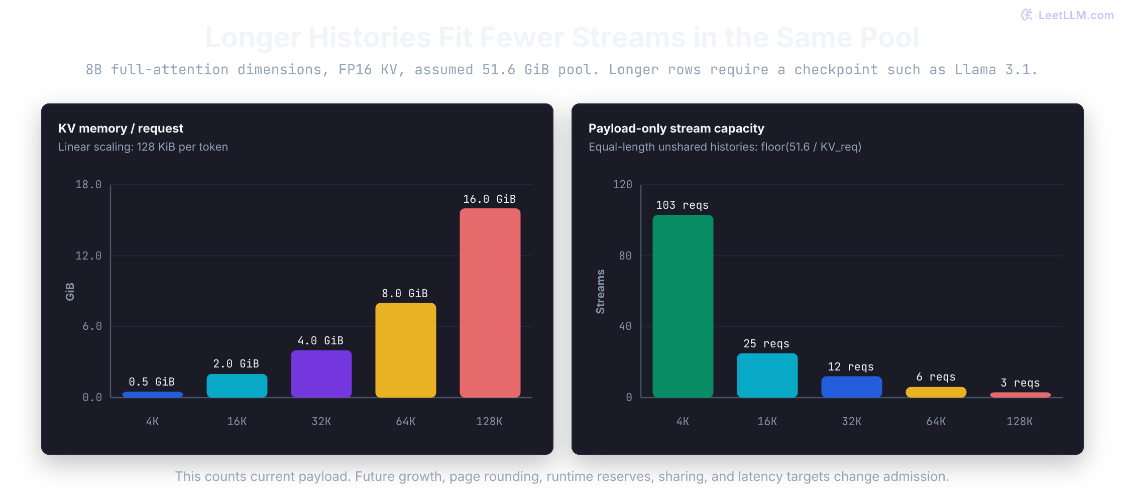
Assume a 51.60 GiB pool, derived from an explicit byte budget below. The 8B dimensions give these capacities. For the longer rows, use a checkpoint such as Llama 3.1 8B that supports 128K.[5] The original April Llama 3 8B has an 8K limit.[7] Matching memory geometry doesn't extend a model's supported context.
| Sequence length () | KV per request (FP16) | Max concurrent streams () | Concurrency drop |
|---|---|---|---|
| 4,096 tokens (4K) | 0.50 GiB | 103 requests | Baseline |
| 16,384 tokens (16K) | 2.00 GiB | 25 requests | -76% |
| 32,768 tokens (32K) | 4.00 GiB | 12 requests | -88% |
| 65,536 tokens (64K) | 8.00 GiB | 6 requests | -94% |
| 131,072 tokens (128K) | 16.00 GiB | 3 requests | -97% |
Before flooring, payload capacity scales as . The 128K row fits three streams, rather than proving a particular tokens/s rate. A fourth independent full-payload request can't join that snapshot; it must wait, be rejected, or cause another request to be preempted. A serving policy chooses among those outcomes.
def kv_cache_gib(
    batch_size: int,
    seq_len: int,
    num_layers: int,
    num_kv_heads: int,
    head_dim: int,
    dtype_bytes: int = 2,
) -> float:
    dimensions = (batch_size, seq_len, num_layers, num_kv_heads, head_dim, dtype_bytes)
    if any(type(value) is not int or value <= 0 for value in dimensions):
        raise ValueError("all dimensions and dtype_bytes must be positive integers")
    total_bytes = (
        2 * batch_size * seq_len * num_layers * num_kv_heads * head_dim * dtype_bytes
    )
    return total_bytes / (1024 ** 3)

one_8k = kv_cache_gib(1, 8_192, 80, 8, 128)
batch_64 = kv_cache_gib(64, 8_192, 80, 8, 128)

print(f"Llama 3 70B, one 8K request: {one_8k:.1f} GiB")
print(f"64 active 8K requests: {batch_64:.0f} GiB")
print("single-request estimate correct:", one_8k == 2.5)
print("64-request estimate correct:", batch_64 == 160.0)
assert kv_cache_gib(1, 4_096, 32, 8, 128) == 0.5
assert kv_cache_gib(2, 8_192, 80, 8, 128) == 2 * one_8k
try:
    kv_cache_gib(1, -1, 80, 8, 128)
except ValueError:
    pass
else:
raise AssertionError("negative sequence length accepted")Llama 3 70B, one 8K request: 2.5 GiB
64 active 8K requests: 160 GiB
single-request estimate correct: True
64-request estimate correct: TrueThat 160 GiB figure assumes every request occupies a live 8K payload. A max-context slab reservation is far worse: it reserves memory for tokens that never arrive.
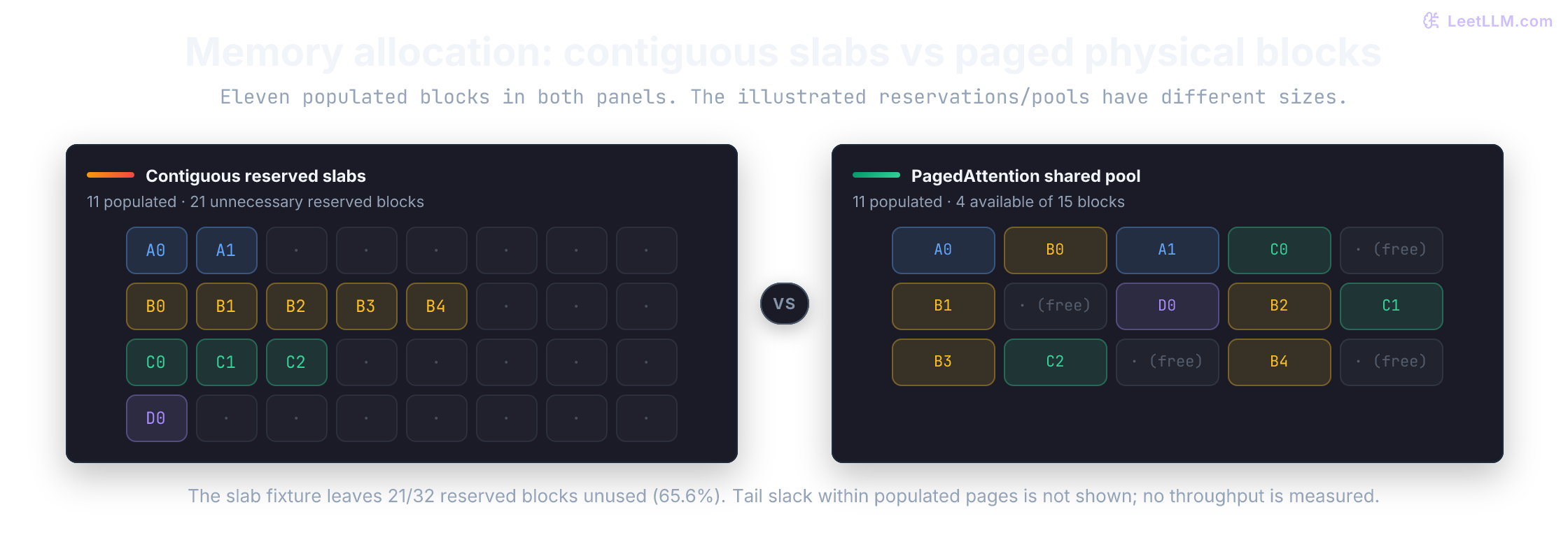
PagedAttention allocates fixed-size blocks (e.g. 16 tokens) as needed and maps logical order through a block table.[8] Exclusively owned pages become reusable after their readers finish; shared or cached pages need separate ownership/eviction accounting. Paging avoids maximum-length reservations without shrinking live-token payload. A partial last block wastes at most fifteen slots here, not universally less than 4%: a one-token history wastes 15/16 slots, or 93.75%.
In the KV-cache formula, which terms can the serving stack change without shortening user context?
Answer
KV-cache quantization reduces the stored bytes per element, with scale metadata and quality trade-offs. Admission changes batch size. For a fixed checkpoint, KV-head count, layer count, and head dimension are architectural constants; choosing a GQA/MQA model is a model choice.
The throughput, latency, cost triangle
Once bandwidth and KV residency are in view, "maximize tokens per second" is not a complete objective. Start with the product promise: interactive users care about TTFT and p95 ITL, while offline batch jobs care about completion throughput and cost per token.
Larger batches amortize weight reads. They also bring more KV history and arithmetic into each iteration. The roughly 4.8 ms calculation is an ideal weight serialization floor, not a measured decode duration or evidence that sixteen requests cost the same as one.
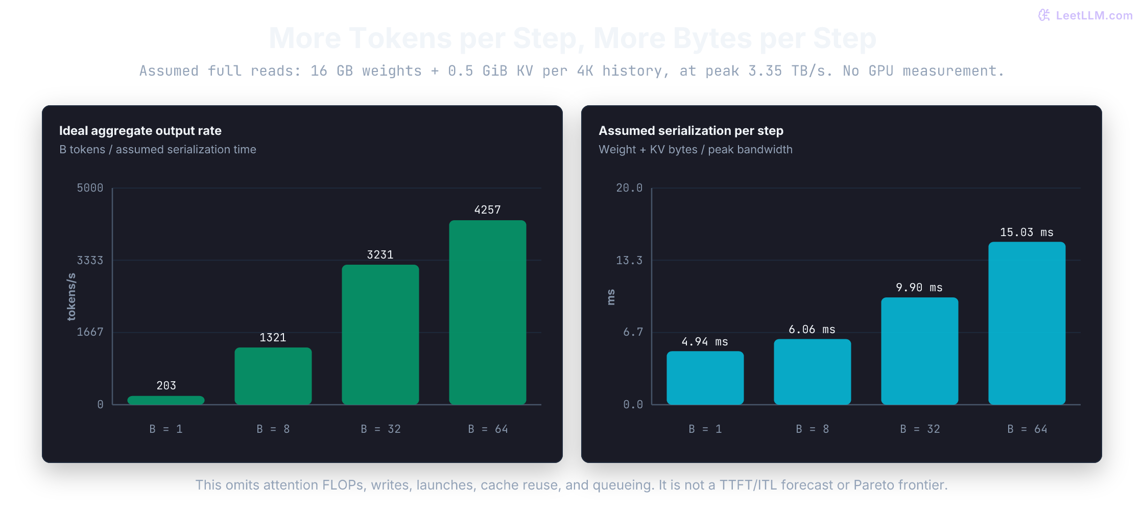
Try an explicit full-read thought experiment: 16 GB of weights plus 0.5 GiB of KV per active 4K history, all read once from HBM per step at peak 3.35 TB/s. Exclude attention FLOPs, writes, launches, cache reuse, and queueing. The assumed byte cost already makes step duration rise with batch size:
weight_bytes = 16_000_000_000
kv_per_request = 2 * 4096 * 32 * 8 * 128 * 2
peak_bytes_per_second = 3.35e12
linear_flops_per_token = 2 * 8_000_000_000

for batch in (1, 8, 32, 64):
    bytes_read = weight_bytes + batch * kv_per_request
    seconds = bytes_read / peak_bytes_per_second
    intensity = batch * linear_flops_per_token / bytes_read
    print(f"B={batch}: {seconds * 1000:.2f} ms, {batch / seconds:.1f} tokens/s, {intensity:.1f} linear FLOPs/byte")
print("Assumed full reads at peak bandwidth; not measured GPU results.")B=1: 4.94 ms, 202.6 tokens/s, 1.0 linear FLOPs/byte
B=8: 6.06 ms, 1320.5 tokens/s, 6.3 linear FLOPs/byte
B=32: 9.90 ms, 3230.9 tokens/s, 15.4 linear FLOPs/byte
B=64: 15.03 ms, 4257.4 tokens/s, 20.3 linear FLOPs/byte
Assumed full reads at peak bandwidth; not measured GPU results.At B=64, the parameter-dependent work has intensity about 20.3 FLOPs/byte in this model, rather than the weight-only estimate of 64. Actual attention adds FLOPs, and actual layouts/cache reuse change traffic. Neither formula is a substitute for profiling. The useful question is which bytes and operations your estimate omitted.
In a live endpoint, inspect three additional pressures:
- KV reads and arithmetic can increase iteration duration as membership and history grow.
- Mixed prefills, transfers, and client buffering can change token gaps.
- Offered arrivals beyond sustainable service capacity build queues unless work is rejected or expired. KV exhaustion may cause waiting or preemption, depending on policy.
| Objective | Typical lever | Trade-off |
|---|---|---|
| Throughput (tokens/s across replica) | Amortize reads with effective batches | More resident history/work can increase per-step latency |
| Lower latency (TTFT, p95 ITL) | Bound work, queue wait, and prompt interference | May leave capacity unused; measure the arrival mix |
| Lower cost per useful token | Sustain quality/SLO-qualified output per billed interval | Include idle time, retries, other workers, and fixed costs |
The GPU-only cost component is hourly GPU spend divided by sustained output. It excludes CPU/network/storage and other service costs. Use useful, quality-qualified output if that is the product's objective:
Treat $3.00/hour as an arithmetic fixture, not a cloud quote. Suppose a replica sustains 2,500 output tokens/s across active requests over the billed interval, including prompt processing and idle periods:
- Tokens per hour = 2,500 * 3,600 = 9,000,000
- Cost per million tokens = $3.00 / 9,000,000 * 1,000,000 = $0.33
At 250 output tokens/s, it rises to $3.33. Latency constraints can justify that gap, but throughput alone doesn't identify the cause: low demand or an inefficient runtime can also produce it.
import math

def cost_per_million(hourly_cost: float, sustained_tps: int) -> float:
    if (not math.isfinite(hourly_cost) or hourly_cost < 0
            or type(sustained_tps) is not int or sustained_tps <= 0):
        raise ValueError("cost must be finite/nonnegative; throughput a positive integer")
    cost = hourly_cost / (sustained_tps * 3600) * 1_000_000
    if not math.isfinite(cost):
        raise ValueError("reported cost overflowed")
    return cost

well_batched = cost_per_million(3.00, 2_500)
starved = cost_per_million(3.00, 250)

print(f"2,500 tokens/s: ${well_batched:.2f} per million tokens")
print(f"250 tokens/s: ${starved:.2f} per million tokens")
print(f"cost multiplier: {starved / well_batched:.0f}x")2,500 tokens/s: $0.33 per million tokens
250 tokens/s: $3.33 per million tokens
cost multiplier: 10xA missing price encoded as NaN must not become a reported cost. The helper rejects nonfinite financial inputs instead of passing them into a dashboard:
for malformed_price in (float("nan"), float("inf")):
    try:
        cost_per_million(malformed_price, 250)
    except ValueError:
        pass
    else:
        raise AssertionError("nonfinite price became a reported cost")
print("missing/infinite prices rejected")missing/infinite prices rejectedOptimized kernels or schedulers can improve throughput and latency together. A Pareto frontier contains measured configurations where improving one objective requires worsening another, under the same workload and comparison contract. There is no universal B=32–64 sweet spot. Find feasible configurations under your latency and quality targets, then compare their cost.
| Operating point | Batch pressure | Cost per token | Latency profile | Workload fit |
|---|---|---|---|---|
| Latency-first | Limit mixed-step work and waiting | Can be higher if fewer tokens amortize spend | Must meet measured TTFT/ITL targets | Chat, autocomplete |
| Balanced | Fit admission to the measured workload | Compare feasible cost points | Check tails by request class | Assistant endpoints |
| Throughput-first | Keep sustained useful work available | Can be lower with good amortization | Accept the workload's completion targets | Offline batch, evaluations |
Production tip: Watch KV occupancy, prefill backlog, queue age, and HBM bandwidth together. High KV occupancy plus preemptions suggests a residency limit. Low KV occupancy and idle compute may mean low demand, a CPU bottleneck, or bandwidth-bound decode; they don't by themselves prove that a larger batch is available.
Two teams serve the same 8B model on the same GPU SKU but report a 5x gap in cost per million tokens. The interactive team is more expensive. Why isn't that automatically a misconfiguration?
Answer
Interactive serving caps batch size to protect TTFT and ITL, so each GPU-hour spreads over fewer tokens. The batch team pushes until throughput saturates. Both can be correct operating points for their SLOs.
Batching raises arithmetic intensity
The previous chapter treated continuous batching as slot reuse: when request A finishes, D can enter at the next decode iteration instead of waiting for C's long answer.[9] Slot reuse is only half the story. One decode step still streams the weight tensor roughly once for the whole batch. More active tokens on that step means more useful FLOPs per byte, which is how serving climbs the roofline without changing the model.
Static batching fights that climb. If three assistant requests need 2, 2, and 5 remaining tokens, a request-level batch of size 3 spends later steps on padding or idle slots. Iteration-level scheduling keeps the weight read attached to live work.
Predict the comparison before running it: finished slots should admit new work sooner. Both policies receive the same five requests with remaining lengths [2, 2, 5, 3, 1] and three slots. This sketch counts decode iterations as idealized full-weight reads, not milliseconds. Prompts are assumed already processed; there are no prefill costs, KV limits, arrivals, or kernel timing.
from collections import deque

lengths = [2, 2, 5, 3, 1]
static_steps = max(lengths[:3]) + max(lengths[3:])
static_tokens = sum(lengths)

queue = deque([2, 2, 5, 3, 1])
active: list[int] = []
max_batch = 3
weight_reads = 0
emitted = 0

while queue or active:
    while queue and len(active) < max_batch:
        active.append(queue.popleft())
    if not active:
        break
    weight_reads += 1
    nxt: list[int] = []
    for remaining in active:
        remaining -= 1
        emitted += 1
        if remaining > 0:
            nxt.append(remaining)
    active = nxt

print(f"static batch: {static_tokens} tokens in {static_steps} weight reads")
print(f"continuous batch: {emitted} tokens in {weight_reads} weight reads")
print(f"tokens per weight read (static): {static_tokens / static_steps:.2f}")
print(f"tokens per weight read (continuous): {emitted / weight_reads:.2f}")
assert emitted == static_tokens == 13
assert (static_steps, weight_reads) == (8, 5)static batch: 13 tokens in 8 weight reads
continuous batch: 13 tokens in 5 weight reads
tokens per weight read (static): 1.62
tokens per weight read (continuous): 2.60Both policies emit 13 tokens. Static batching takes five iterations for the first group, then three for the second. Continuous batching starts the last two requests after iteration two and finishes everything in five iterations. That's fewer idealized weight reads, not a measured 8/5 speedup: real step duration changes with membership and context length. Admitting past the cache budget can instead trigger eviction or preemption.
Why does batching help decode even though every request still needs its own next token?
Answer
The model weights can be read once for a larger set of active tokens, so that memory movement is amortized across requests. Batching doesn't remove the sequential dependency inside each request. It raises useful work per weight read until KV memory or latency SLOs say stop.
Sharing, chunking, and phase isolation
Three more levers change the same budget without training a new model. Each targets a different source of pressure: repeated prompt work, prompt interference, or movement between phase-specific workers.
Reuse identical prefixes
Many assistant requests start from the same system prompt. Prefix caching is the lookup that finds reuse across independent requests.
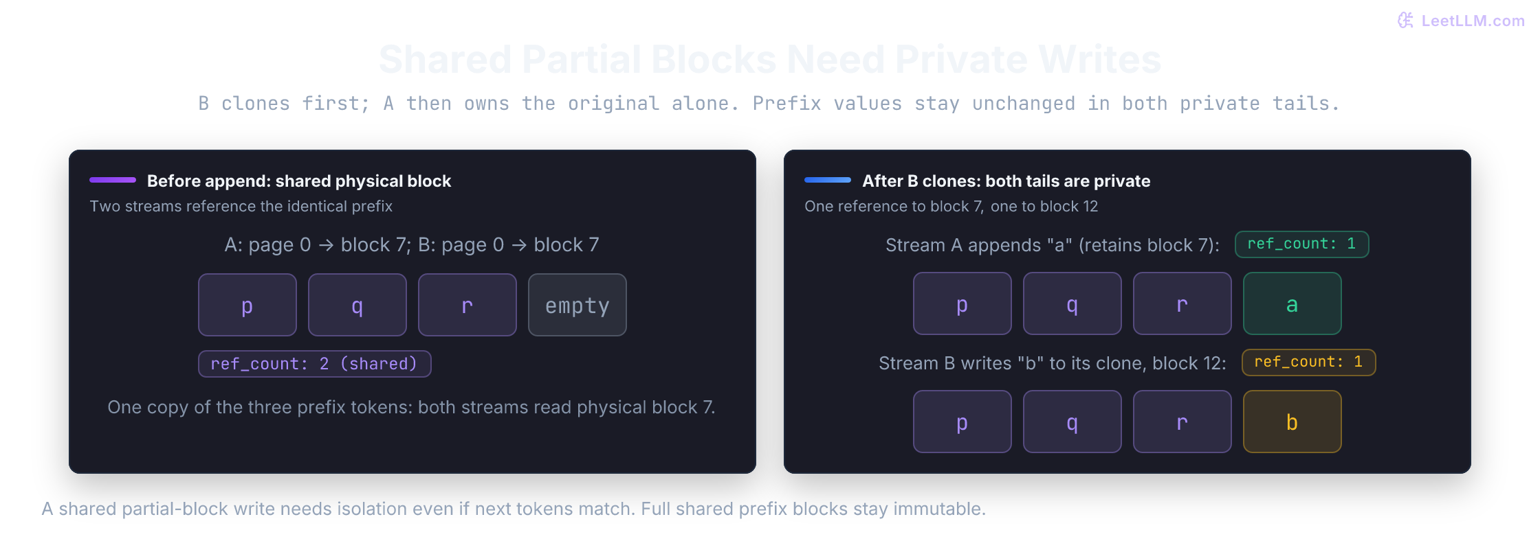
Copy-on-write protects shared state: if two continuations share a partially filled block, a writer first clones that block before appending to it.[8] Existing prefix tokens aren't edited. A full shared block stays immutable, and new tokens go into private tail blocks. Independent prefix caches often reuse only full blocks, so they needn't clone a partial block on every hit.
For Llama 3 8B, an identical 4K prefix has a 0.5 GiB KV payload stored once if sharing is supported. Each later session still needs metadata, private continuation KV, and decode attention over that prefix. Reuse requires identical effective model state, token IDs and positions, plus an appropriate tenant-isolation policy. It saves prefix computation and duplicate storage, not all subsequent attention work.
Bound prompt interference
A 10K RAG prompt on the same worker as live streams can increase token gaps. SARATHI studies combining chunked prefills with decode work.[10] Checked October 10, 2026: vLLM V1 enables chunked prefill when possible, prioritizes pending decode work, then spends remaining max_num_batched_tokens budget on prompt chunks.[11]
Chunking doesn't add HBM or guarantee smoother delivery. Smaller mixed iterations can reduce interference, but extra boundaries/context work can increase prefill cost. Remeasure TTFT and ITL together; details live in the scheduling chapter.
Separate phases when transfer is worth paying
Splitwise and DistServe move prefill and decode onto separate pools when avoided interference or better resource allocation pays for KV transfer.[12][1] This changes worker placement, not payload size.
For a Llama 3 70B 8K request, payload is 2.5 GiB. At an assumed effective one-way rate of 200 GiB/s, serializing the whole payload takes at least 12.5 ms before protocol and scheduling. This isn't a named interconnect specification. Overlap, sharding, contention, and already-cached blocks change the transfer's critical-path cost. In a simple non-overlapped comparison, the split must save more time than transfer plus coordination adds.
kv_cache_gib = 2.5  # Llama 3 70B, one 8K request
interconnect_gib_s = 200  # binary GiB/s

ideal_transfer_ms = kv_cache_gib / interconnect_gib_s * 1000
mixed_ms = (kv_cache_gib * 1024**3) / (200 * 1_000_000_000) * 1000

print(f"KV state to transfer: {kv_cache_gib:.1f} GiB")
print(f"ideal one-way floor at {interconnect_gib_s} GiB/s: {ideal_transfer_ms:.1f} ms")
print(f"mixed GiB / decimal-GB/s floor (for comparison): {mixed_ms:.1f} ms")
print("Queueing saved must exceed transfer plus protocol and scheduling overhead.")KV state to transfer: 2.5 GiB
ideal one-way floor at 200 GiB/s: 12.5 ms
mixed GiB / decimal-GB/s floor (for comparison): 13.4 ms
Queueing saved must exceed transfer plus protocol and scheduling overhead.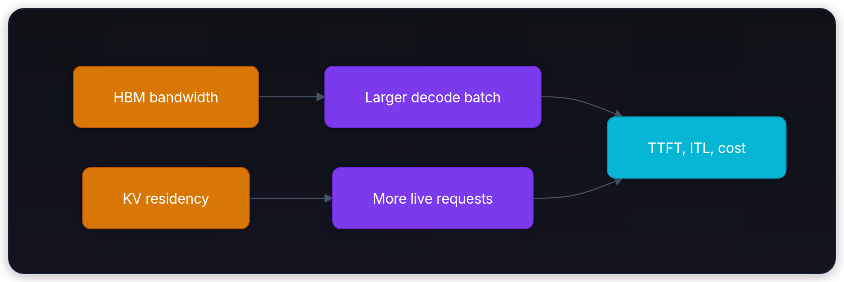
Bandwidth sets how hard you can push the batch. KV residency sets how many requests that batch can contain. The operating point is where those two ceilings meet the product's latency SLO.
When can prefill-decode disaggregation make latency worse?
Answer
When KV-cache transfer, coordination, or extra scheduling cost more than the head-of-line blocking they remove. Short prompts, light traffic, or a slow interconnect often favor a colocated worker.
Speculative decoding buys tokens per weight read
Batching amortizes one target-model weight read across concurrent requests. Speculative decoding applies the same insight within a single stream: one target weight read can verify several sequential future tokens.[13]
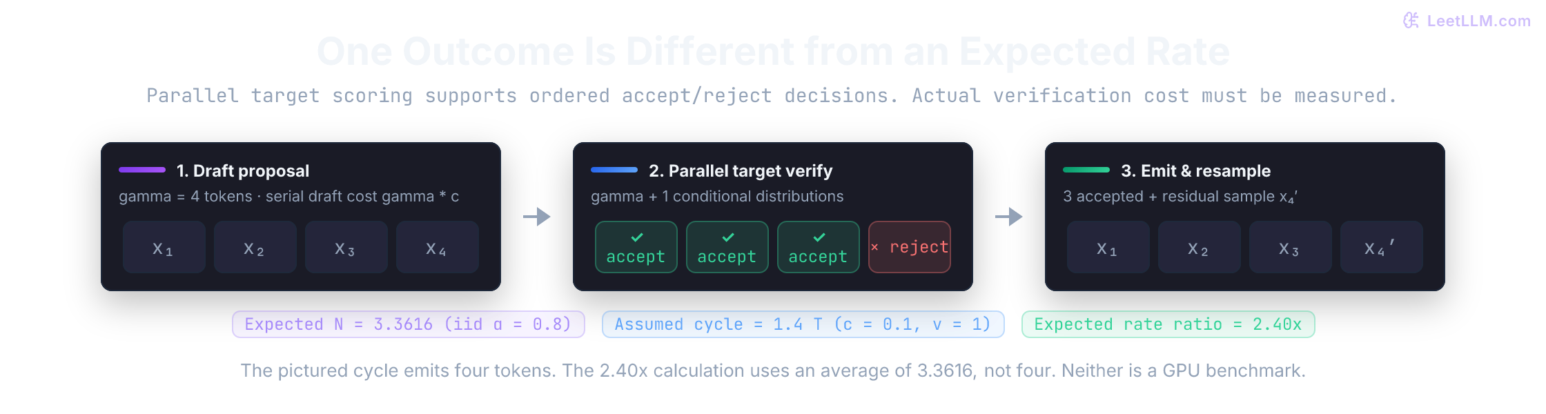
In the classic algorithm, a draft model proposes candidate tokens. Target verification supplies conditional distributions: one for each proposal and one for a possible concluding token.[13] A causal forward pass can evaluate the drafted prefixes together; cached logits and runtime layout determine how many new input positions it schedules. Parallel verification is not automatically as cheap as ordinary one-token decode.
Let be draft-step cost relative to ordinary target decode. Measure it; parameter-count ratios don't determine it. Let be verification plus remaining cycle overhead in the same units. For serial draft generation followed by verification:
Acceptance decisions follow proposal order, using scores already computed by verification. For a proposal actually sampled from , use target distribution conditioned on the same prefix. Both distributions include the intended sampling transformations, such as temperature or top-p.[13] Accept with probability:
On the first rejection at position , the remaining draft tokens are discarded, and the engine immediately samples a replacement token from the normalized positive residual distribution:
If all proposals survive, sample an extra token from the target distribution conditioned on the accepted prefix. The ideal algorithm emits 1 through tokens before stopping/truncation and preserves the intended target distribution, not an identical seeded sequence. Real finite-precision implementations require their own numerical and sampling checks.
The paper's geometric expectation assumes acceptance rates are independent and identically distributed, with mean .[13] Under that assumption, the probability that the first proposals all survive is . A fleet-wide mean alone doesn't establish those survival probabilities. Add the concluding correction/bonus sample:
For , the limit is . Compare the resulting expected rate with ordinary target decode, assuming long enough generations and the costs above:
For an assumed , , , and iid acceptance mean :
The expectation predicts 3.36 tokens per cycle costing 1.40 baseline-step units, or a rate ratio. It isn't a measured speedup or the outcome of one cycle.
Now consider the failure mode: if the draft model struggles on code or dense reasoning, and acceptance drops to while draft cost is :
The modeled token rate is about 11% lower; time per token is about 12% higher, since it scales as the reciprocal. The break-even condition for this serial cost model is . Acceptance, span length, and verification overhead must be measured together.
import random
import math

def validate_dist(dist: list[float], vocab: int) -> None:
    if len(dist) != vocab or any(not math.isfinite(x) or x < 0 for x in dist):
        raise ValueError("invalid distribution entries")
    if not math.isclose(sum(dist), 1.0, abs_tol=1e-9):
        raise ValueError("distribution must sum to one")

def sample(dist: list[float], rng: random.Random) -> int:
    cutoff = rng.random() * sum(dist)
    running = 0.0
    for i, mass in enumerate(dist):
        running += mass
        if cutoff < running:
            return i
    return max(i for i, mass in enumerate(dist) if mass > 0)

def residual_sample(p: list[float], q: list[float], rng: random.Random) -> int:
    leftover = [max(pt - qt, 0.0) for pt, qt in zip(p, q)]
    total = sum(leftover)
    if total <= 0:
        raise ValueError("rejection requires positive residual mass")
    return sample(leftover, rng)

def speculative_step(
    draft_tokens: list[int],
    draft_dists: list[list[float]],
    target_dists: list[list[float]],
    rng: random.Random,
) -> list[int]:
    k = len(draft_tokens)
    if len(draft_dists) != k or len(target_dists) != k + 1:
        raise ValueError("need k draft and k+1 target distributions")
    vocab = len(target_dists[0])
    if vocab == 0:
        raise ValueError("empty vocabulary")
    for dist in draft_dists + target_dists:
        validate_dist(dist, vocab)
    for token, q in zip(draft_tokens, draft_dists):
        if type(token) is not int or not 0 <= token < vocab or q[token] <= 0:
            raise ValueError("draft token must have positive proposal probability")
    accepted: list[int] = []
    for i, token in enumerate(draft_tokens):
        p = target_dists[i]
        q = draft_dists[i]
        if rng.random() < min(1.0, p[token] / q[token]):
            accepted.append(token)
            continue
        return accepted + [residual_sample(p, q, rng)]
    return accepted + [sample(target_dists[k], rng)]

def speculative_speedup(gamma: int, alpha: float, c: float, verify_cost: float = 1.0) -> float:
    if (type(gamma) is not int or gamma < 1
            or not all(math.isfinite(value) for value in (alpha, c, verify_cost))
            or not (0 <= alpha <= 1 and c >= 0 and verify_cost > 0)):
        raise ValueError("invalid parameters for speculative speedup")
    expected_tokens = (1 - alpha ** (gamma + 1)) / (1 - alpha) if alpha < 1.0 else float(gamma + 1)
    cycle_cost = gamma * c + verify_cost
    if not math.isfinite(cycle_cost):
        raise ValueError("cycle cost overflowed")
    return expected_tokens / cycle_cost

rng = random.Random(0)
draft_tokens = [0, 1]
draft_dists = [[0.8, 0.2], [0.3, 0.7]]
target_dists = [[0.7, 0.3], [0.2, 0.8], [0.4, 0.6]]
emitted = speculative_step(draft_tokens, draft_dists, target_dists, rng)

print(f"emitted tokens: {emitted}")
assert emitted == [0, 1, 1]
rejected = speculative_step([0], [[1.0, 0.0]], [[0.0, 1.0], [0.5, 0.5]], random.Random(1))
assert rejected == [1]
assert speculative_step([0], [[1.0, 0.0]], [[1.0, 0.0], [0.0, 1.0]], random.Random(1)) == [0, 1]
try:
    speculative_step([1], [[1.0, 0.0]], [[0.5, 0.5], [0.5, 0.5]], random.Random(1))
except ValueError:
    pass
else:
    raise AssertionError("impossible draft token accepted")
print(f"forced rejection emits: {rejected}")

speedup_fast = speculative_speedup(4, 0.8, 0.1)
speedup_slow = speculative_speedup(4, 0.3, 0.15)
print(f"speedup (gamma=4, alpha=0.8, c=0.1): {speedup_fast:.2f}x")
print(f"speedup (gamma=4, alpha=0.3, c=0.15): {speedup_slow:.2f}x")
assert math.isclose(speedup_fast, 2.401, abs_tol=0.01)
assert speedup_slow < 1.0
print("acceptance, rejection, speedup multipliers, and invalid support checked")emitted tokens: [0, 1, 1]
forced rejection emits: [1]
speedup (gamma=4, alpha=0.8, c=0.1): 2.40x
speedup (gamma=4, alpha=0.3, c=0.15): 0.89x
acceptance, rejection, speedup multipliers, and invalid support checkedKeep verification cost explicit. Predict what happens to the same acceptance profile if verification takes twice the ordinary target step:
for malformed_gamma, malformed_cost in ((2.5, 0.1), (4, float("inf"))):
    try:
        speculative_speedup(malformed_gamma, 0.8, malformed_cost)
    except ValueError:
        pass
    else:
        raise AssertionError("invalid span/cost accepted")
print(f"verification cost 1T: {speculative_speedup(4, 0.8, 0.1):.2f}x")
print(f"verification cost 2T: {speculative_speedup(4, 0.8, 0.1, verify_cost=2):.2f}x")
print("fractional spans and infinite draft costs rejected")verification cost 1T: 2.40x
verification cost 2T: 1.40x
fractional spans and infinite draft costs rejectedWith this seed both drafts survive, so the first call emits two accepted tokens plus one extra. The second call rejects a proposal with zero target probability and emits its residual correction. Boundary checks aren't a proof of distributional exactness, but they prevent the acceptance-only demo from hiding a broken rejection branch. Follow-on methods such as EAGLE use a lightweight feature-level drafting network informed by target hidden states.[14]
Serving question stays the same: did accepted tokens repay the extra draft and verification work?
Why can speculative decoding be exact yet still slower than normal decoding?
Answer
The accept/reject rule can preserve the target distribution, but runtime depends on acceptance and overhead. If the draft is wrong too often, or verification is expensive, saved target passes don't cover the extra work.
Lower precision cuts the bytes in that read
If decode repeatedly streams weights and past KV states, reducing precision is the most direct hardware bandwidth lever. The key is distinguishing which memory stream you are compressing: static model weights or dynamic KV cache buffers.
Many production stacks begin with BF16 or FP16, then adopt FP8 execution when modern accelerators (like NVIDIA Hopper or Ada Lovelace) provide native FP8 Tensor Cores, or use weight-only INT4/INT8 formats (such as AWQ or GPTQ) when the primary goal is shrinking decode memory traffic.[15][16]
Weight quantization: shifting decode toward the compute roof
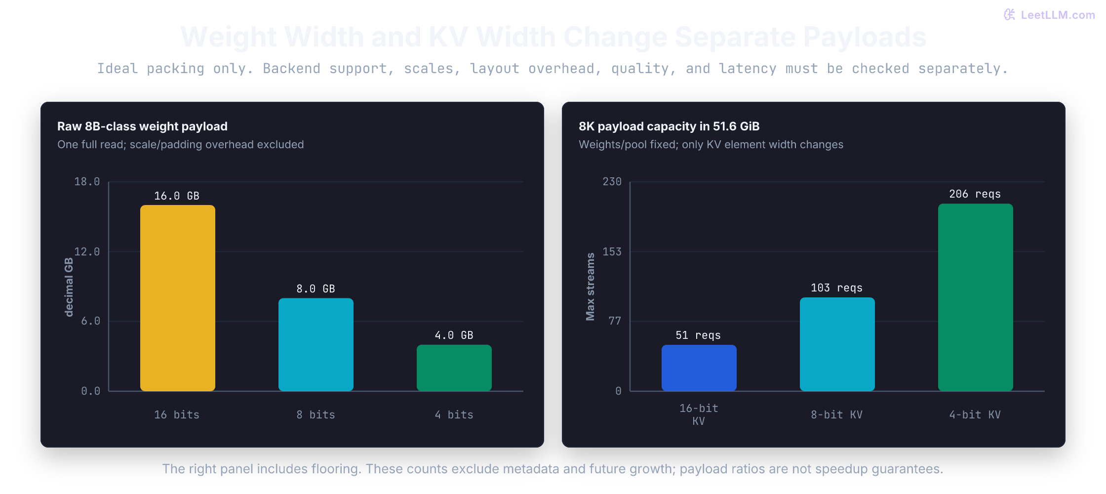
When weight reads dominate, moving an ideal 8B payload from FP16 (2 bytes/parameter) to an 8-bit format (1 byte) or packed INT4 (0.5 byte) reduces it from 16 GB to 8 GB or 4 GB. Scales, padding, unquantized tensors, and kernel layouts add to those payloads:
- Serialization: 4 GB / 3,350 GB/s is about 1.2 ms versus 4.8 ms for 16 GB. These are full-read floors at peak bandwidth, not decode timings or a guaranteed fourfold speedup.
- Intensity: The weight-only formula increases fourfold at the same batch. KV traffic, dequantization, and the compatible compute format change the complete roofline. B=75 with INT4 doesn't prove tensor-core saturation.
- Capacity: Saving 12 decimal GB releases about 11.18 GiB. If all of it can join the unchanged KV pool, the fixture's 4K payload capacity rises from 103 to 125, adding 22 streams before scales, output growth, or latency limits. It doesn't add 24 half-GiB histories.
Keep the batch and histories fixed to isolate traffic. In the earlier full-read model, 64 requests with 4K histories read about 34.36 decimal GB of KV per iteration, already more than the 16 GB weights. Quartering the weights doesn't quarter the combined read. Predict the result when histories grow to 16K:
batch = 64
fp16_weights, int4_weights = 16_000_000_000, 4_000_000_000
kv_bytes_per_token = 2 * 32 * 8 * 128 * 2
for history in (4096, 16384):
    kv_read = batch * history * kv_bytes_per_token
    before = fp16_weights + kv_read
    after = int4_weights + kv_read
    # Same achieved bandwidth, full KV reads, unchanged batch and cache width.
    traffic_rate_ratio = before / after
    assert 1 < traffic_rate_ratio < 4
print(f"history={history}: KV read={kv_read / 1e9:.2f} GB; rate ratio={traffic_rate_ratio:.2f}x")history=4096: KV read=34.36 GB; rate ratio=1.31x
history=16384: KV read=137.44 GB; rate ratio=1.08xThis yields about 1.31× at 4K and 1.08× at 16K for the assumed bandwidth-only rate, before dequantization or any other overhead. The 64-stream 16K case needs 128 GiB of raw KV, so it exceeds our earlier single-GPU pool; it is a traffic extrapolation for sufficient storage, not a feasible admission setting on that replica. Profile the actual read mix before choosing weight compression, KV compression, or a smaller retained history. Recompute the model if weight savings instead fund a larger batch.
KV cache quantization: doubling concurrency and slashing attention bandwidth
KV precision is a separate choice from weight precision, though an execution mode can also quantize queries or other operations. Current vLLM FP8 documentation describes backend-specific schemes, scale calibration, and leaving selected layers unquantized.[17] Formats such as INT8/INT4 require their own supported model/backend path. Compare two ideal payload effects:
- Capacity: One byte rather than two halves raw 8B KV from 128 KiB to 64 KiB/token. Flooring prevents exact stream-count doubling: a fixed 51.6 GiB pool's 8K payload capacity goes from 51 to 103, before scale/layout overhead. At 128K it goes from 3 to 6. Admission and SLO-qualified capacity may differ.
- Traffic: If each active request's full retained K/V payload is read once from HBM, the model's byte count is: Whether it exceeds weight traffic depends on batch, architecture, and history. Halving element width halves this raw term, not bandwidth as a device property or measured ITL. Cache reuse, repeated loads, scales, conversion, and other work change the realized benefit. Evaluate output quality too.
import math

parameters = 8_000_000_000
bytes_per_weight = {"FP16": 2.0, "INT8": 1.0, "INT4": 0.5}

for precision, width in bytes_per_weight.items():
    traffic_gb = parameters * width / 1_000_000_000
    print(f"{precision}: {traffic_gb:.1f} GB of weights per full read")

print("INT4 weight traffic is 0.25x FP16 before kernel overhead.")
pool_gib = (80_000_000_000 - 16_000_000_000) / 1024**3 - 8
freed_gib = 12_000_000_000 / 1024**3
old_capacity = math.floor(pool_gib / 0.5)
new_capacity = math.floor((pool_gib + freed_gib) / 0.5)
print(f"12 decimal GB released: {freed_gib:.2f} GiB")
print(f"4K raw KV capacity: {old_capacity} -> {new_capacity} (+{new_capacity - old_capacity})")
assert (old_capacity, new_capacity) == (103, 125)FP16: 16.0 GB of weights per full read
INT8: 8.0 GB of weights per full read
INT4: 4.0 GB of weights per full read
INT4 weight traffic is 0.25x FP16 before kernel overhead.
12 decimal GB released: 11.18 GiB
4K raw KV capacity: 103 -> 125 (+22)Common mistake: 4-bit weights aren't primarily an artifact to save disk space. The real serving win is fewer bytes transferred across the memory bus during each decode step. Whether that translates to lower user-facing latency still depends on kernel dequantization overhead and whether model accuracy passes your evaluations.
Why does weight-only INT4 often help decode latency more directly than prefill latency?
Answer
Decode repeatedly streams model weights for small per-token work, so fewer bytes per weight cut bandwidth pressure. Prefill uses larger matrix operations and can be compute-heavy, so weight compression isn't always the dominant lever there.
When one request no longer fits
The 8B replica was a fit-and-batch problem. To stress-test the formula, extrapolate the 70B architecture to 1,000,000 cached tokens: 2 * 1_000_000 * 80 * 8 * 128 * 2 bytes, about 305 GiB. This is hypothetical memory arithmetic, not a supported Llama context length. The original Llama 3 release supports 8K and Llama 3.1 extends it to 128K.[7][5] Sharding memory doesn't extend a checkpoint's trained positional behavior.
That isn't a "buy one more H100" situation. One request has crossed the single-device residency boundary.
Context parallelism (CP) splits the sequence dimension across devices, not the layer stack or the batch. Each GPU holds a shard of the prompt and its KV.
Attention still needs information from other shards. Ring Attention is one approach for long-sequence processing: while a device computes blockwise attention on local queries, K/V blocks rotate around the ring.[18] Decode implementations can instead combine partial attention results across cache shards. The communication pattern depends on phase and implementation; don't assume every system circulates all KV on each generated token.
That isn't tensor parallelism, which shards work and weights inside a layer, or pipeline parallelism, which shards layers. These techniques can be combined, and tensor parallelism may also shard KV heads.
Llama 3 70B in FP16 is about 140 GB of parameters, so it can't reside on one 80 GB GPU even at batch 1.[5] The next chapter, model parallelism, makes that split its main subject.
def kv_gib(sequence_tokens: int) -> float:
    total_bytes = 2 * sequence_tokens * 80 * 8 * 128 * 2
    return total_bytes / 1024**3

total_kv = kv_gib(1_000_000)
devices = 4
print(f"hypothetical 1M-token KV with 70B dimensions: {total_kv:.1f} GiB")
print(f"evenly sharded over {devices} devices: {total_kv / devices:.1f} GiB/device")
print("KV only: weights, communication buffers, and runtime need additional memory.")hypothetical 1M-token KV with 70B dimensions: 305.2 GiB
evenly sharded over 4 devices: 76.3 GiB/device
KV only: weights, communication buffers, and runtime need additional memory.What bottleneck does context parallelism target, and what bottleneck can it introduce?
Answer
It targets per-request context and KV that no longer fit on one GPU. It can introduce communication overhead because devices must exchange partial attention state across sequence shards.
When the budget lies
These traces show up when formulas look fine on paper but users or profiles disagree. Start with the symptom, name the ceiling it points to, then test one targeted fix.
"I bought a higher-FLOP GPU and decode barely moved"
Peak compute went up, but tokens per second didn't. That observation alone doesn't identify the bottleneck. Profile HBM, kernels, transfers, and host scheduling. If full reads saturate bandwidth while tensor compute has headroom, test amortization or fewer bytes before expecting extra peak FLOPs to help.
"Throughput is up and chat feels worse"
Aggregate TPS rose after you lifted max batch, but users report sluggish streams. Inspect iteration duration, queue wait, and delivery by request class; mean TPOT can hide gaps. Gate on the product's TTFT and ITL targets, not replica tokens/s alone. Separate traffic classes if their interference is the measured problem.
"Speculative decoding added latency"
A draft model is in the path, and p50 decode got worse. Acceptance may be too low, or draft-plus-verify overhead may exceed the saved target passes. Measure accepted tokens per draft span before rollout. If most proposals die early, keep ordinary decode.
"HBM climbs even though every session shares a system prompt"
KV usage looks close to batch * full_prompt despite repeated text. Copy-on-write isolates writes after sharing is established; it doesn't discover matching prefixes. Cross-request prefix caching needs a compatible available entry and trusted sharing scope. Branching inside one request can share directly. Inspect allocated pool bytes separately from live/cached block ownership, then confirm actual reuse and reference counts.
A dashboard shows high TTFT, a rising prefill backlog, stable TPOT, and moderate KV memory. Which subsystem should you inspect first?
Answer
Inspect prefill scheduling and admission first. Stable TPOT suggests decode isn't currently degrading, while high TTFT plus a prefill backlog points to prompt work or queueing before the first token.
Size the 8B replica
Put the pieces together with an explicit accounting budget. This simplified partition includes reserved/unavailable space in the last term; real engines have more detailed categories:
For this fixture, account for:
- Weights: Approximate the 8B-class FP16 payload as bytes, or 14.90 GiB. The exact checkpoint, packing, adapters, and execution path determine its real allocation.
- KV pool: Physical storage from which requests use blocks. A preallocated pool can keep the same device allocation while live block ownership grows or shrinks.
- Activations/workspace: Intermediate tensors, kernel scratch, and captured-graph buffers depend on model, batch/chunk shapes, dtype, and backend. FlashAttention avoids the full score/probability intermediates; it doesn't remove all workspace. Measure the peak rather than assume 2–4 GiB universally.
- Other allocations/reserve: Runtime allocations, allocator slack, other GPU users, and intentionally unused headroom. Host scheduling queues aren't automatically VRAM allocations. vLLM's
gpu_memory_utilizationlimits the model executor's fraction, rather than specifying a fixed activation/slack split; explicitkv_cache_memory_bytesoverrides automatic pool sizing.[19]
GB means bytes; GiB means bytes. Assume exactly 80,000,000,000 budget bytes here, or 74.51 GiB. Don't infer the runtime's available byte count from a nominal “80 GB” product label; inspect device-reported total/free memory and engine allocations. Subtract the approximate weights and an assumed 8 GiB combined workspace/other reserve:
Now compute single-request payload for a 4,096-token sequence on Llama 3 8B:
KV bytes = 2 * 1 * 4096 * 32 * 8 * 128 * 2
         = 536,870,912 bytes
         = 0.50 GiB
The theoretical payload ceiling is:
That snapshot counts 4,096 retained positions per request with no future growth. Reserve 512 more positions, giving 4,608 positions or 0.5625 GiB per request, and this fixture's growth-budget ceiling drops to:
Average context lengths aren't admission guarantees: a sudden burst of long prompts can exhaust physical blocks even if the historical average was 4K.
import math

kv_bytes = 2 * 1 * 4_096 * 32 * 8 * 128 * 2
kv_per_request_gib = kv_bytes / 1024**3
device_gib = 80_000_000_000 / 1024**3
weight_gib = 16_000_000_000 / 1024**3
runtime_gib = 8
kv_budget_gib = device_gib - weight_gib - runtime_gib
arithmetic_ceiling = math.floor(kv_budget_gib / kv_per_request_gib)
growth_gib = (4_096 + 512) * (2 * 32 * 8 * 128 * 2) / 1024**3
growth_ceiling = math.floor(kv_budget_gib / growth_gib)

print(f"KV per 4K request: {kv_per_request_gib:.2f} GiB")
print(f"KV budget after weights and runtime: {kv_budget_gib:.2f} GiB")
print(f"arithmetic-only batch ceiling: {arithmetic_ceiling}")
print(f"ceiling with 512 output tokens reserved: {growth_ceiling}")
assert arithmetic_ceiling == 103 and growth_ceiling == 91
assert 91 * growth_gib <= kv_budget_gib < 92 * growth_gibKV per 4K request: 0.50 GiB
KV budget after weights and runtime: 51.60 GiB
arithmetic-only batch ceiling: 103
ceiling with 512 output tokens reserved: 91Why isn't that 103-request snapshot a safe production max concurrency?
Answer
It counts current payload, not future output growth, page rounding, or workload tails. The runtime reserve is an assumption and latency may fail much earlier. Reserving 512 more tokens already lowers this fixture to 91 requests before measuring any SLO.
Try a page-aware admission calculation next. Use 16-token blocks, count each request's prompt plus reserved output, and sum the rounded allocations. For prompts [4090, 4096, 4100] with 512 reserved output tokens each, predict whether three times the average length gives the exact allocation.
BYTES_PER_TOKEN = 2 * 32 * 8 * 128 * 2
BLOCK_TOKENS = 16

def reserved_bytes(prompt_tokens: int, output_tokens: int) -> int:
    if (type(prompt_tokens) is not int or type(output_tokens) is not int
            or prompt_tokens <= 0 or output_tokens < 0):
        raise ValueError("use integer counts: prompt positive, output reserve nonnegative")
    blocks = (prompt_tokens + output_tokens + BLOCK_TOKENS - 1) // BLOCK_TOKENS
    return blocks * BLOCK_TOKENS * BYTES_PER_TOKEN

prompts = [4090, 4096, 4100]
allocations = [reserved_bytes(prompt, 512) for prompt in prompts]
payload = sum(prompt + 512 for prompt in prompts) * BYTES_PER_TOKEN
reserved = sum(allocations)
assert reserved >= payload
assert reserved - payload < len(prompts) * BLOCK_TOKENS * BYTES_PER_TOKEN
assert reserved_bytes(4096, 512) < reserved_bytes(4097, 512)
print("reserved token slots:", [value // BYTES_PER_TOKEN for value in allocations])
print("unused rounded slots:", (reserved - payload) // BYTES_PER_TOKEN)

def admit(current_bytes: int, new_request_bytes: int, budget_bytes: int) -> bool:
    return current_bytes + new_request_bytes <= budget_bytes

exact_fit = admit(sum(allocations[:2]), allocations[2], reserved)
too_small = admit(sum(allocations[:2]), allocations[2], reserved - 1)
assert exact_fit and not too_small
print("last request fits exact budget:", exact_fit)
print("last request fits one byte less:", too_small)reserved token slots: [4608, 4608, 4624]
unused rounded slots: 18
last request fits exact budget: True
last request fits one byte less: FalseThe answer is 4,608, 4,608, and 4,624 slots: 18 unused slots in total. The last prompt crosses a page boundary. This calculation deliberately excludes shared prefixes and cache eviction; it models a conservative reservation for these requests, not a complete allocator. On a serving engine, verify peak allocated memory, preemptions, TTFT, and token-gap percentiles under mixed-length load before turning such a calculation into an admission limit.