Personalize this lesson
Adapt explanations and teaching visuals to your background and preferred voice.
On Thursday evening, a cluster's forecast for Friday was 132 outbound batch jobs. Friday's observed count was 160. Is that 28-job gap a capacity problem, a planned launch, or a broken counter?
Ranking and recommendation compared items for a query or user. Here the order that matters is time: forecasting predicts a later count from information already available, while anomaly detection checks whether the eventual gap deserves investigation. We'll forecast one day ahead, compare two simple baselines, and turn an unusually large error into a review with enough context to investigate it.
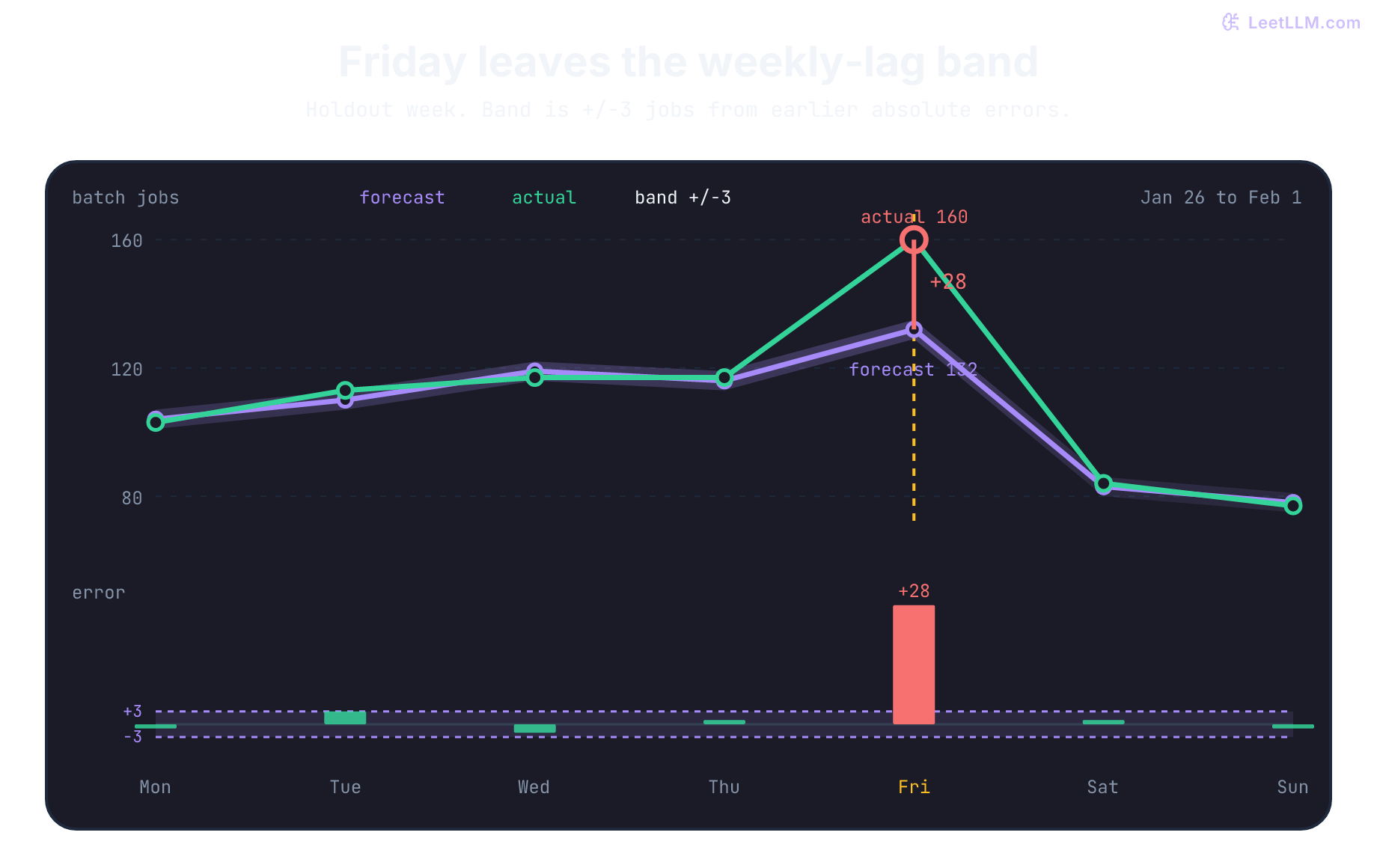
160 − 132 = +28 forecast error crosses an empirical +/-3 band. The other six days stay inside. The band comes from earlier errors, not a guaranteed future coverage rate.Start with an ordered batch-job series
Before naming a model, fix the clock. A time series is a sequence of observations indexed by time. Here, each row is one day's outbound batch-job count for one model-serving cluster, plus a flag for a planned model launch. Friday's 160 versus 132 gap is one row in that ordered sequence.
The forecast horizon is how far ahead you predict. A one-day horizon targets tomorrow; issuing a full seven-day forecast targets horizons one through seven. Those are different evaluation tasks, even if a simple baseline happens to return the same numbers.
This lab issues one forecast each evening for the following day, assuming today's final count is available then. The end of that evening is the forecast origin. A Sunday forecast for Monday may use Sunday's count; a forecast issued the previous Thursday may not. In production, delayed telemetry can move the latest usable observation further back.
Use this synthetic four-week series throughout. Its weekday pattern repeats with small changes, and the final Friday contains a planned launch. The launch flag is assumed known before the forecast, although this baseline doesn't use it to adjust the predicted count. Every later cell continues in the same Python session.
from datetime import date, timedelta
from hashlib import sha256
from json import dumps
from math import ceil, sqrt

start = date(2026, 1, 5)
weekly_pattern = [100, 112, 115, 118, 132, 82, 76]
weekly_noise = [
    [0, 0, 0, 0, 0, 0, 0],
    [2, -2, 3, -2, 2, 2, 2],
    [4, -2, 4, -2, 0, 1, 2],
    [3, 1, 2, -1, 28, 2, 1],
]

rows = []
for week, noise in enumerate(weekly_noise):
    for weekday, (baseline, offset) in enumerate(zip(weekly_pattern, noise)):
        rows.append(
            {
                "date": start + timedelta(days=7 * week + weekday),
                "weekday": weekday,
                "volume": baseline + offset,
                "launch_event": week == 3 and weekday == 4,
            }
        )

print("rows:", len(rows))
print("first date:", rows[0]["date"])
print("last date:", rows[-1]["date"])
print("launch_event day:", next(row["date"] for row in rows if row["launch_event"]))rows: 28
first date: 2026-01-05
last date: 2026-02-01
launch_event day: 2026-01-30The fixture contains one row per calendar day. The seven-row lag below only means seven days because there are no missing dates. Real ingestion should validate the calendar, timezone, and missing-day policy; a missing measurement isn't automatically a zero count.
Decompose metrics into trend, seasonality, and exogenous events
A decomposition is a modeling choice, not a unique identification of physical causes. One useful additive description is:[1]
Interpret these terms as descriptions of the observed pattern:
- Trend (): A changing underlying level. Adoption might increase demand, but four authored weeks don't establish a long-run trend.
- Seasonality (): Repeating calendar effects. Our daily series has a weekly pattern. Daily aggregates don't reveal hourly cycles, and month-end effects need more than a seven-day seasonal lag.
- External effect (): A modeled contribution from covariates such as planned launches or holidays. The launch flag isn't itself an additive number of jobs. Its effect would have to be estimated from earlier examples, or supplied as an explicit scenario.
- Remainder (): Everything not explained by those terms, including measurement errors, omitted structure, and shocks. It isn't automatically independent random noise.
Autoregressive dependence is another way to model predictable history, rather than a separately identified term in this decomposition. A backlog can persist; that doesn't prove all workloads have high lag-1 correlation.
The structural formulation above is additive. It suits seasonal swings that stay roughly constant in absolute magnitude. When those swings scale proportionally with the level (such as weekend traffic dropping by 35% rather than a flat forty jobs), a multiplicative description may suit them better:
Here is a multiplicative remainder and the components must be suitable for that product. Taking logs of positive values converts products into sums and can stabilize proportional variation. It doesn't guarantee constant error variance. Zero counts require another choice, such as log1p, whose interpretation differs. Back-transforming a predicted log mean also needs a bias adjustment to obtain an original-scale mean; exponentiation alone doesn't supply it.
Keep future rows out of training
A random split answers a different question from forecasting. Suppose we issue a forecast for January 6. If the training set contains January 31, the model has already seen later demand, seasonal behavior, or a launch event relative to that target. The split can look balanced while the evaluation is still optimistic.
The audit compares the latest training date with the earliest test date. Alternating rows between train and test creates the same time-order problem as shuffling. Predict future_leak=True for these interleaved rows and future_leak=False for the chronological rows.
interleaved_train = list(range(0, len(rows), 2))
interleaved_test = list(range(1, len(rows), 2))
time_train = list(range(21))
time_test = list(range(21, 28))

def split_summary(name, train_indices, test_indices):
    latest_train = max(rows[index]["date"] for index in train_indices)
    earliest_test = min(rows[index]["date"] for index in test_indices)
    future_leak = latest_train >= earliest_test
    print(
        f"{name}: latest_train={latest_train} "
        f"earliest_test={earliest_test} future_leak={future_leak}"
    )

split_summary("interleaved", interleaved_train, interleaved_test)
split_summary("time-aware", time_train, time_test)
assert max(time_train) < min(time_test)interleaved: latest_train=2026-01-31 earliest_test=2026-01-06 future_leak=True
time-aware: latest_train=2026-01-25 earliest_test=2026-01-26 future_leak=FalseThis is a single chronological holdout, not yet cross-validation. Later we'll move the forecast origin and evaluate repeated future targets, which is time-series cross-validation.[1] The date check is necessary but not sufficient: feature values, transformations, and event flags must also reflect what was known at each origin. A table sorted by date can still contain features computed from future observations.
Why isn't a random split acceptable just because every row belongs to the same cluster?
Answer
Cluster identity doesn't remove time order. A shuffled split can train on later demand, launch events, and seasonal behavior before evaluating earlier dates. Production only predicts later periods from earlier information.
Establish a same-weekday baseline
On Sunday evening, January 25, the latest count is 78; last Monday's was 104. Tomorrow will actually run 103 jobs, but the forecaster doesn't know that yet. Which observed value is the better starting point for Monday?
Put the two one-step copies beside the actual count:
| Method | What it copies | Monday forecast | Actual | Error |
|---|---|---|---|---|
| naive | yesterday (Sunday 78) | 78 | 103 | +25 |
| seasonal naive | last Monday (104) | 104 | 103 | -1 |
The mismatch has a name: batch-job volume has seasonality when a pattern repeats at a known calendar frequency. Saturday volume stays lower than weekday volume, so copying yesterday turns a weekend lull into Monday's forecast.
A seasonal naive forecast reuses the observation from the matching previous season. For daily data with a weekly pattern, Monday copies last Monday, Tuesday copies last Tuesday, and so on.[1] It's a benchmark, not a claim that the world is simple. A more complex model has to beat it on later windows before its extra machinery is worth running.
For the two days that matter most, the same-weekday rule gives:
| Target day | Same day last week | Forecast | Actual | Forecast error |
|---|---|---|---|---|
| Monday, Jan 26 | Monday, Jan 19 | 104 | 103 | -1 |
| Friday, Jan 30 | Friday, Jan 23 | 132 | 160 | +28 |
Read Friday's row as 160 - 132 = 28. Positive error means observed volume exceeded the forecast; negative error means the forecast was too high.
The table shows two rows. Now compute the complete holdout week, with every forecast reading the value exactly seven rows earlier. Before running the cell, predict Monday's -1 and Friday's +28.
holdout = list(range(21, 28))

def weekly_lag(index, origin=None):
    origin = index - 1 if origin is None else origin
    source = index - 7
    if not 0 <= source <= origin < index:
        raise ValueError("Weekly lag needs an observed matching day before the target")
    return rows[source]["volume"]

for index in holdout:
    forecast = weekly_lag(index)
    actual = rows[index]["volume"]
    error = actual - forecast
    print(
        f"{rows[index]['date']} forecast={forecast} "
        f"actual={actual} error={error:+d}"
)2026-01-26 forecast=104 actual=103 error=-1
2026-01-27 forecast=110 actual=113 error=+3
2026-01-28 forecast=119 actual=117 error=-2
2026-01-29 forecast=116 actual=117 error=+1
2026-01-30 forecast=132 actual=160 error=+28
2026-01-31 forecast=83 actual=84 error=+1
2026-02-01 forecast=78 actual=77 error=-1Saturday exposes the same trap in the other direction. A naive one-step forecast would copy Friday's launch (160) into Saturday and miss by -76. The weekly lag copies last Saturday (83) and misses by +1, because it preserves the weekend regime.
Freeze issuance at Sunday, January 25, instead of advancing it daily. A seven-row copy can forecast horizons one through seven from already observed sources. Horizon eight would read Monday, January 26, which hasn't happened at this origin:
frozen_origin = 20
print("horizon seven forecast:", weekly_lag(frozen_origin + 7, origin=frozen_origin))
try:
    weekly_lag(frozen_origin + 8, origin=frozen_origin)
except ValueError:
print("horizon eight reads an unobserved source: rejected")horizon seven forecast: 78
horizon eight reads an unobserved source: rejectedA general multi-step seasonal-naive rule repeats the last observed season for longer horizons. Our simple helper deliberately rejects a source beyond its origin instead of silently reading a future row.
Why is last Monday a better forecast for this Monday than yesterday's Sunday count?
Answer
Sunday is a weekend lull. Copying 78 into Monday treats that dip as the new baseline and misses by 25 jobs. Last Monday already lived in the weekday regime, so the error is 1 job.
Compare classical SARIMAX, gradient-boosted trees, and foundation models
Our same-weekday baseline misses the known launch. Could another model learn its effect? Compare candidates that use the information available at issuance, rather than choosing complexity from a leaderboard. These families offer different ways to share history and represent covariates.
Classical SARIMAX
SARIMAX combines regression with seasonal ARIMA structure. In the regression-with-SARIMA-errors formulation used by statsmodels, with fixed coefficients and no intercept shown:[2]
Here shifts a series back one observation, is the seasonal period, and is a covariate vector. Differencing applies to the regression error , not simply to while leaving the regressors unchanged on the right. Differencing can remove particular trends or seasonal unit roots; it doesn't cure every form of nonstationarity. The AR and MA polynomials describe dependence on past errors and innovations.
Low-order models can be compact, with model-based prediction intervals under their distributional assumptions. Coefficients describe conditional associations, not necessarily causal launch effects. Future covariates must be supplied as known values or forecasts; uncertain covariates add uncertainty the usual conditional interval may omit.
A conventional statsmodels SARIMAX fit has one target series. Fitting it independently for 25,000 containers creates 25,000 local models without learned cross-container sharing. That is a trade-off of this setup, not a theorem forbidding shared parameters, pooled statistical models, or multivariate state-space alternatives.
Gradient-boosted trees with rolling features
LightGBM and XGBoost are options for turning forecasting into supervised tabular regression.[3][4] For a one-step target at , issued after , inputs might include:
- Autoregressive lag features: Exact historical values at .
- Rolling summary statistics: Mean, standard deviation, minimum, and maximum over windows ending at , using only observations available at issuance.
- Cyclical calendar encodings: Trigonometric projections of day of week () and hour of day.
- Categorical metadata: Cluster GPU architecture, tenant tier, and deployment region.
A global model can pool rows across series and use metadata to learn shared relationships. Validate temporal feature joins, per-series weighting, cold-start performance, and runtime; pooling doesn't guarantee useful transfer or effortless scale.
Now let denote the origin. Common ways to predict include:
- Recursive forecasting: Train a one-step model. Feed its prediction back into lag features for later steps. Errors can propagate and predicted inputs can differ from the observed inputs used in training.
- Direct forecasting: Fit a separate model for each horizon using origin-available features. This avoids feeding earlier predicted targets into later lags, but doesn't eliminate forecast error. A shared model with horizon as an input, or a multiple-output model, offers other trade-offs.
A holiday calendar may be known at . Actual weather at isn't; a weather forecast issued at is a different, potentially usable input.
Time-series Transformers and foundation models
Numerical time series can become Transformer tokens in several ways. One token per timestamp gives dense attention an attention-map cost in sequence length ; patching changes the token count. Neither tokenization nor a larger pretrained model guarantees better forecasts.
Distinguish these methods and generations:
- PatchTST (ICLR 2023): Embeds patches and shares encoder weights across independently processed channels. With patch length , stride , and the paper's end padding, the token count is , approximately , not generally . Dense attention maps cost per channel. Independence omits explicit channel interaction; it isn't a guarantee against noise or negative transfer.[5]
- Original Chronos (2024): Mean-scales historical values and uses uniformly spaced bins, not quantile bins, in the reported experiments. Primarily T5-based models learn cross-entropy on quantized sequences and sample future tokens autoregressively. This isn't the architecture of every later Chronos release.[6]
- Chronos-2 (released October 20, 2025): Uses continuous patch embeddings, alternating time/group attention, and quantile outputs. It supports multivariate targets and past-only or known-future covariates without task-specific training.[7]
- TimesFM-3 (released August 31, 2026): Adds native multivariate targets and covariates, alternates temporal and variate attention, and fills masked future patches in one forward pass. Its reported outputs include quantiles from P10 to P90; don't treat P90 as an available P99 estimate.[8]
These capabilities were checked October 10, 2026. Zero-shot means no task-specific fitting; forecasting still uses supplied context and the model's supported inputs. It doesn't mean a brand-new cluster needs no observations, or that generated quantiles are calibrated on your traffic. Compare later-window accuracy, interval coverage, and actual serving cost against the same issuance schedule and baselines.
Try the PatchTST arithmetic before choosing a context length:
lookback, patch_length, stride = 336, 16, 8
without_padding = (lookback - patch_length) // stride + 1
with_paper_padding = without_padding + 1
print("un-padded patches:", without_padding)
print("paper-padded patches:", with_paper_padding)
print("raw / patched attention-map entries:", lookback**2 / with_paper_padding**2)un-padded patches: 41
paper-padded patches: 42
raw / patched attention-map entries: 64.0The 64× ratio counts entries in one attention map. Projection layers, channel count, memory movement, and hardware determine runtime; it isn't a measured 64× speedup.
Measure forecast error in batch jobs
The holdout errors are -1, 3, -2, 1, 28, 1, -1. Their signed average is 29 / 7 = 4.1, which measures average underforecasting, not typical error magnitude. Negative and positive errors can cancel, so we also want the average size of each mistake.
Mean absolute error (MAE) averages that size without letting positive and negative errors cancel:[1]
Here is the number of evaluated days, is observed volume on day , and is the forecast for that day. For the holdout week, the absolute weekly-lag errors are 1, 3, 2, 1, 28, 1, 1. Their sum is 37, so MAE is 37 / 7 = 5.3 batch jobs.
MAE stays in batch jobs, which operations can read. It treats a 28-job miss and a 28-job surplus as equal, though underforecasting a capacity spike may cost more. When that asymmetry matters, keep MAE and record a separate business-cost measure.
Calculate overall MAE and normal-day MAE separately. The second metric excludes the known launch-event day so one planned spike doesn't hide weekday behavior. Before running the cell, predict overall MAE 5.3, normal-day MAE 1.5, and yesterday's-lag MAE 23.6.
def mean_absolute_error(errors):
    return sum(abs(error) for error in errors) / len(errors)

holdout_errors = [
    rows[index]["volume"] - weekly_lag(index)
    for index in holdout
]
normal_errors = [
    rows[index]["volume"] - weekly_lag(index)
    for index in holdout
    if not rows[index]["launch_event"]
]

naive_errors = [
    rows[index]["volume"] - rows[index - 1]["volume"]
    for index in holdout
]

print("holdout errors:", holdout_errors)
print("holdout MAE:", round(mean_absolute_error(holdout_errors), 1))
print("normal-day MAE:", round(mean_absolute_error(normal_errors), 1))
print("naive holdout MAE:", round(mean_absolute_error(naive_errors), 1))holdout errors: [-1, 3, -2, 1, 28, 1, -1]
holdout MAE: 5.3
normal-day MAE: 1.5
naive holdout MAE: 23.6The weekly lag's MAE is 5.3 jobs versus 23.6 for yesterday's lag. Both are daily one-step forecasts: Tuesday's naive forecast may use Monday's newly observed count. A seven-day forecast issued on Sunday would instead repeat Sunday's count for every naive prediction. Don't compare those two issuance schedules as though they were the same task.
Keep the overall metric alongside the non-launch slice. Excluding a difficult day can help diagnose the model, but it doesn't remove the capacity cost of missing that day. Choose slices before examining which exclusions improve the score.
Backtest more than one future window
A single future week can make a baseline look lucky. Rolling-origin evaluation moves the forecast origin forward and scores the next target each time. Here we group those daily one-step errors into two reporting windows: January 19 through January 25, then January 26 through February 1. These aren't two fixed-origin seven-step forecasts.
Run both folds. The seasonal baseline can forecast each day because each starts after at least one full week of history. Predict the result before running: the earlier fold should be calmer than the launch-containing fold.
folds = []
for window_start in (14, 21):
    indices = list(range(window_start, window_start + 7))
    errors = [
        rows[index]["volume"] - weekly_lag(index, origin=index - 1)
        for index in indices
    ]
    fold = {
        "start": rows[indices[0]]["date"],
        "end": rows[indices[-1]]["date"],
        "mae": round(mean_absolute_error(errors), 1),
    }
    folds.append(fold)
print(f"{fold['start']} to {fold['end']}: MAE={fold['mae']}")2026-01-19 to 2026-01-25: MAE=0.9
2026-01-26 to 2026-02-01: MAE=5.3The two folds disagree for a reason: the later window contains the launch spike. Keep that context instead of collapsing it into one global average. Backtest by model-serving cluster, service tier, weekday, and launch-event status so a cluster that routinely underforecasts peak demand stays visible.
These two weeks demonstrate the backtest, not stable performance across seasons. Keep model or threshold tuning inside earlier validation windows, then evaluate a later untouched period. Our earlier reporting fold will also contribute to interval calibration below, so it isn't an independent test of that fitted interval. For a learned model, refit on an expanding history or recent rolling window at each chosen origin; this copy rule has no coefficients to refit.
Also match the target to the decision. Job count only approximates GPU demand if job sizes are comparable. GPU-hours, queue-delay duration, or failed-job count may be more appropriate for other operational decisions.
Distinguish forecast errors from residuals
The next question is what each subtraction means. Two related quantities often get called residuals. Hyndman and Athanasopoulos separate them on two axes: which rows they use and how many steps ahead they look.[1] Use the row source and forecast timing to keep the labels straight:
| Quantity | Which rows | How far ahead | Formula | What it tells you |
|---|---|---|---|---|
| residual | training data after fitting | usually one-step fitted values | observed value minus fitted value | whether the model captured known history |
| forecast error | later data, after the forecast was issued | one-step or multi-step | observed value minus forecast | whether the model predicted unseen future data |
Friday's +28 is a forecast error because Friday's observed volume wasn't available when the forecast was issued. This weekly-lag baseline has no fitted parameters, so a one-step training residual uses the same copy-last-week rule.
The rule stays constant; the evidence changes. Training residuals describe known history, while forecast errors test a later window. An operations team may casually say "residual alert," but the stored artifact should name the measured quantity.
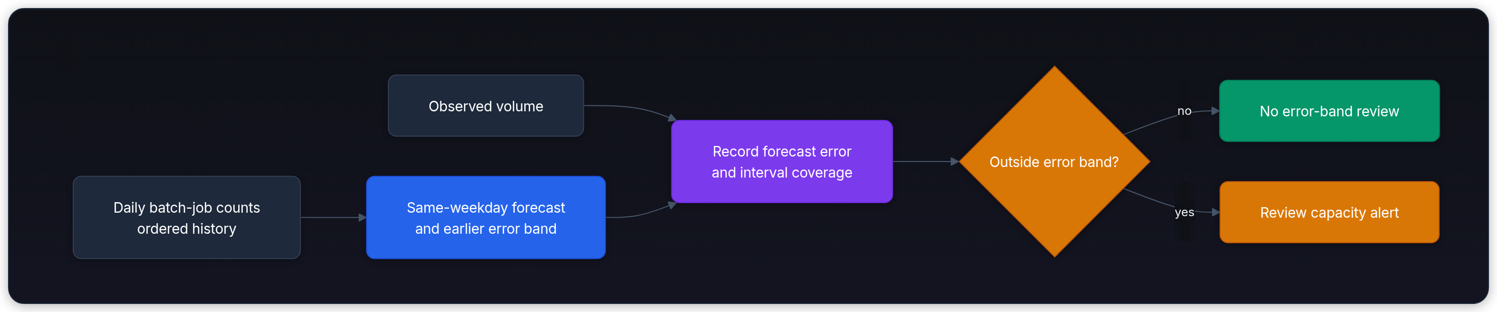
The flow now needs one more boundary: how wide is normal? An unusual forecast error can trigger review, but it can't tell us whether Friday's cause was a launch, bad telemetry, or genuine demand.
Quantify uncertainty with pinball loss and conformal intervals
A point forecast doesn't specify its exceedance probability. The mean and median needn't coincide, and neither job counts nor a demand quantile directly determines server capacity when job sizes vary.
- P10: A low demand quantile. Provisioning to it can underprovide for most outcomes; it doesn't ensure safe teardown.
- P50: A median. It isn't generally the expected demand needed for mean-based cost accounting.
- P90 or P99: Higher demand quantiles that can inform headroom decisions. They don't guarantee an SLA, and some models don't produce P99.
Lead time, queue tolerance, resource-per-job variation, and the cost of spare capacity also matter. An unexpected change can invalidate even a previously calibrated quantile.
Quantile regression with pinball loss
To predict a specific quantile without assuming a normal distribution, models optimize the asymmetric pinball loss (also called check loss):
Examining the two piecewise linear slopes reveals how it works:
- When actual demand exceeds the forecast (, underforecasting), the error is positive, incurring penalty .
- When actual demand falls below the forecast (, overforecasting), the error is negative, incurring penalty .
For , underpredicting by ten jobs incurs loss 9.0; overpredicting by ten incurs 1.0. Minimizing expected conditional pinball loss targets a conditional quantile. A finite, restricted, imperfectly optimized model needn't reach it. For counts and other distributions with atoms, ties mean a quantile needn't have exactly 10% of outcomes strictly above it.[9]
Consider ten equally likely demand outcomes: nine at ten jobs, one at 100. Their mean is 19, but only one outcome exceeds 19. At q=0.9, every prediction between ten and 100 minimizes this discrete example's expected loss. Check both claims:
demand = [10] * 9 + [100]

def pinball(actual, predicted, quantile):
    error = actual - predicted
    return max(quantile * error, (quantile - 1) * error)

mean_demand = sum(demand) / len(demand)
print("mean demand:", mean_demand)
print("fraction above mean:", sum(value > mean_demand for value in demand) / len(demand))
print("ten-job underforecast loss:", pinball(20, 10, 0.9))
print("ten-job overforecast loss:", round(pinball(10, 20, 0.9), 1))
for prediction in (10, 19, 100):
    expected_loss = sum(pinball(value, prediction, 0.9) for value in demand) / len(demand)
print(f"prediction {prediction}: expected P90 loss={expected_loss:.1f}")mean demand: 19.0
fraction above mean: 0.1
ten-job underforecast loss: 9.0
ten-job overforecast loss: 1.0
prediction 10: expected P90 loss=8.1
prediction 19: expected P90 loss=8.1
prediction 100: expected P90 loss=8.1The canonical inverse-CDF P90 chooses ten, the first value with cumulative probability at least 0.9. This example's pinball-loss optimum isn't unique.
Conformalized prediction intervals
Split conformal prediction can wrap a fitted predictor with a finite-sample marginal coverage guarantee under exchangeability. It doesn't promise coverage for each weekday, cluster, or realized calibration set.[9][10]
On a held-out calibration set , compute absolute residual nonconformity scores . For target coverage (such as 95%, where ), set the interval half-width to the finite-sample adjusted empirical quantile:
Here is the kth smallest score, with no interpolation. The infinity convention handles a requested rank beyond the finite scores. For a predictor fixed independently of calibration data, exchangeable calibration/test scores give , averaging over calibration and the new outcome. Forecasting with dependent rolling history doesn't automatically satisfy those conditions.
The non-exchangeability trap in time series
Ordered traffic with autocorrelation, seasonal changes, or drift needn't have exchangeable scores. An upward shift can make an old band too narrow, but neither the direction nor the size of coverage loss is automatic.[11]
Two approaches worth evaluating are:
- Rolling calibration: Recent scores can track a changing regime, at the cost of fewer observations and noisier quantiles. Choose the window using earlier backtests; rolling fourteen or thirty days doesn't restore exchangeability or a universal 95% guarantee.
- Adaptive conformal inference (ACI): Update a working miscoverage level using . A miss lowers the level, usually widening a monotone interval rule. Its original long-run coverage-frequency result uses specified extreme-set conventions and permits unbounded intervals. It isn't a per-step conditional coverage or useful-width guarantee, and clipping the working level changes the stated algorithm.[12]
Online updates must wait for the outcome to arrive. For delayed daily counts, using tomorrow's realized error to adjust today's interval is leakage. Our lab below uses a frozen empirical band and doesn't implement ACI.
Calibrate an error band from earlier days
A point forecast such as 132 batch jobs leaves an operator with a practical question: how much variation counts as normal? A prediction interval answers by pairing the forecast with lower and upper bounds intended to cover a stated proportion of future outcomes. Hyndman and Athanasopoulos treat the interval as part of the forecast, not a chart decoration, and they evaluate it on later data.[1]
If one-step forecast errors are approximately zero-mean Gaussian with a stable scale, a common approximate 95% interval is . The scale must describe forecast errors at the chosen horizon, not the raw variability of daily volume. A biased forecast or a changing error distribution undermines that interpretation.[1]
We'll use a simpler empirical rule: sort earlier absolute one-day errors and take their nearest-rank 95th percentile as the half-width. This doesn't assume Gaussian errors, but transferring the band to future days still assumes their errors behave sufficiently like the calibration period. It isn't a bootstrap and doesn't account automatically for time dependence.
Calibrate on January 12 through January 25, before the January 26 holdout starts. Then measure coverage again on the later holdout week. Coverage is the share of days whose absolute error stays inside the band.
There are fourteen calibration errors. The nearest-rank index is ceil(0.95 × 14) = 14, so this example selects their largest absolute error, 3. The resulting interval extends three jobs on either side of the forecast, for a total width of six jobs. Always report width alongside coverage; a band that covers everything by becoming enormous isn't useful.
calibration = list(range(7, 21))
calibration_errors = [
    rows[index]["volume"] - weekly_lag(index)
    for index in calibration
]
target_coverage = 0.95
interval_policy = "empirical-absolute-error-p95-v1"

def nearest_rank_quantile(values, probability):
    if not values or not 0 < probability <= 1:
        raise ValueError("Need nonempty values and probability in (0, 1]")
    ordered = sorted(values)
    rank = ceil(probability * len(ordered)) - 1
    return ordered[rank]

error_band = nearest_rank_quantile(
    [abs(error) for error in calibration_errors],
    probability=target_coverage,
)
calibration_coverage = sum(
    abs(error) <= error_band
    for error in calibration_errors
) / len(calibration_errors)
holdout_coverage = sum(
    abs(error) <= error_band
    for error in holdout_errors
) / len(holdout_errors)

error_bias = sum(calibration_errors) / len(calibration_errors)
error_rms = sqrt(sum(error * error for error in calibration_errors) / len(calibration_errors))
normal_half_width = round(1.96 * error_rms, 1)

assert max(calibration) < min(holdout)
print("calibration errors:", calibration_errors)
print("empirical p95 absolute-error half-width:", error_band)
print("mean calibration error:", round(error_bias, 2))
print("root mean squared calibration error:", round(error_rms, 2))
print("zero-mean normal approximation half-width:", normal_half_width)
print("in-sample calibration coverage:", round(calibration_coverage, 3))
print("later holdout coverage:", round(holdout_coverage, 3))calibration errors: [2, -2, 3, -2, 2, 2, 2, 2, 0, 1, 0, -2, -1, 0]
empirical p95 absolute-error half-width: 3
mean calibration error: 0.5
root mean squared calibration error: 1.75
zero-mean normal approximation half-width: 3.4
in-sample calibration coverage: 1.0
later holdout coverage: 0.857The empirical band is +/-3 jobs. The zero-mean normal approximation gives about +/-3.4, so both flag Friday's +28. Neither establishes its cause. The RMS calculation estimates spread around zero; it isn't the sample standard deviation around the observed mean. The positive mean error of 0.5 jobs is a reason to investigate forecast bias rather than silently assume it away.
Neither width is a production 95% guarantee from fourteen calibration errors. Calibration coverage is 1.000 here because the selected order statistic is the maximum. Later holdout coverage is 6 / 7 = 0.857 because Friday falls outside. A single week neither validates a 95% claim nor precisely estimates the policy's long-run coverage.
Compare the ranks directly. With fourteen scores and 95% target coverage, standard split conformal requests ceil(15 × 0.95) = 15, not fourteen. It returns an infinite half-width. Under exchangeable scores with no ties, using the maximum of fourteen gives marginal coverage only 14/15 ≈ 93.3%; ties can raise coverage. Neither result transfers automatically to our time-dependent fixture.
absolute_scores = sorted(abs(error) for error in calibration_errors)
conformal_rank = ceil((len(absolute_scores) + 1) * target_coverage)
conformal_half_width = (
    absolute_scores[conformal_rank - 1]
    if conformal_rank <= len(absolute_scores)
    else float("inf")
)
print("empirical rank:", ceil(len(absolute_scores) * target_coverage))
print("split-conformal rank:", conformal_rank)
print("split-conformal half-width:", conformal_half_width)
print("tie-free maximum coverage:", round(len(absolute_scores) / (len(absolute_scores) + 1), 3))empirical rank: 14
split-conformal rank: 15
split-conformal half-width: inf
tie-free maximum coverage: 0.933Conformal Prediction and Uncertainty develops the guarantee and its assumptions further. Measure later coverage and width across windows, horizons, clusters, and important demand slices before deciding whether an error band is useful.
Even a correctly calibrated 95% interval permits about five misses per hundred predictions on average. Across 1,000 series evaluated daily, that can mean about 50 threshold crossings per day, without implying 50 incidents. Independence isn't needed for that expected count, although dependence affects whether the crossings arrive together.
Why doesn't the tiny +/-3 band prove that future batch-job counts will land inside it 95% of the time?
Answer
It comes from only fourteen earlier errors. In-sample calibration coverage tells you how the band was chosen; later holdout coverage checks whether it transferred to unseen days. One holdout week still isn't enough. A production interval needs enough history plus out-of-sample coverage checks across rolling windows, forecast horizons, and important slices.
Turn an unusual error into a review artifact
The band answers whether Friday is unusual, not why. An anomaly is an observation unusual enough to inspect; it isn't proof that a cluster, pipeline, or model failed. Friday's jump could come from a planned model launch, duplicated event ingestion, a large backfill, or genuine demand growth.
Apply the empirical band to the held-out week. Before running the cell, predict one alert row: Friday's 160 should sit outside [129, 135], with launch_event=True. The alert stores enough context to reproduce that comparison.
forecast_version = "weekly-lag-v1"
policy_cutoff = str(rows[20]["date"])
owner = "capacity-ops"

alerts = []
for index in holdout:
    forecast = weekly_lag(index)
    actual = rows[index]["volume"]
    forecast_error = actual - forecast
    if abs(forecast_error) > error_band:
        alerts.append(
            {
                "series": "fc-a.batch_jobs",
                "forecast_version": forecast_version,
                "policy_cutoff": policy_cutoff,
                "forecast_origin": str(rows[index - 1]["date"]),
                "horizon_days": 1,
                "source_date": str(rows[index - 7]["date"]),
                "interval_policy": interval_policy,
                "date": str(rows[index]["date"]),
                "forecast": forecast,
                "actual": actual,
                "forecast_error": forecast_error,
                "lower": forecast - error_band,
                "upper": forecast + error_band,
                "launch_event": rows[index]["launch_event"],
                "action": "review",
                "owner": owner,
                "resolution": "pending",
            }
        )

for alert in alerts:
    print(f"{alert['date']}: origin={alert['forecast_origin']}, source={alert['source_date']}")
    print(f"forecast={alert['forecast']}, actual={alert['actual']}, "
          f"error={alert['forecast_error']:+d}, band=[{alert['lower']}, {alert['upper']}]")
    print(f"launch_event={alert['launch_event']}, owner={alert['owner']}, "
f"resolution={alert['resolution']}")2026-01-30: origin=2026-01-29, source=2026-01-23
forecast=132, actual=160, error=+28, band=[129, 135]
launch_event=True, owner=capacity-ops, resolution=pendingThe baseline caught Friday because 160 falls outside [129, 135]. A launch-event flag doesn't erase the event; it changes the first investigation step. The comparison says “unusual,” while that flag suggests where to look first.
Route alerts with context. A planned model launch still deserves capacity review. An unexpected deviation deserves investigation too, but surprise alone doesn't make it urgent. Page when there is actionable, time-sensitive impact, such as an exhausted capacity margin or a breached service objective.[13]
def route_alert(alert, urgent_impact=False):
    if urgent_impact:
        return "page actionable capacity impact"
    if alert["launch_event"]:
        return "review planned model launch capacity"
    return "review unexpected batch-job deviation"

for alert in alerts:
print(alert["date"], "->", route_alert(alert))2026-01-30 -> review planned model launch capacityThe policy cutoff is January 25, when the empirical band was fixed. Friday's forecast origin is January 29, and its source observation is January 23. Recording all three distinguishes policy fitting from daily forecast issuance. Neither the historical source date nor the target date substitutes for the origin.
This in-memory receipt illustrates what a later investigation would need. It doesn't issue forecasts on a live clock or persist the observations. A real record also needs issuance timestamps, input versions, telemetry availability, and revisions; a calendar date alone doesn't audit those contracts.
Mitigate alert fatigue with cooldown and multivariate detectors
Detecting threshold crossings is only the first step in monitoring systems. Naive implementations quickly break down under operational scale. Two challenges require structural safeguards: alert fatigue and multi-metric correlation failures.
Alert storms, flapping, and throttling
Four hours of one-minute evaluations gives 240 evaluations. It gives 240 notifications only if every breached evaluation sends one. Separate evaluation, alert state, incident grouping, and notification delivery.
Stateful controls offer distinct trade-offs:
- Persistence: Require repeated breaches before entering alert state. Three samples at five-minute spacing are a configurable policy, not a universal fifteen-minute detection delay. Persistence trades fewer transient notifications for delay and can miss brief real failures.
- Cooldown or deduplication: Update one active alert without sending every evaluation as a new page. An authored sixty-minute cooldown may suit one failure mode; independently urgent symptoms or escalation must still reach the owner.
- Resolution persistence or threshold hysteresis: Require repeated clean samples to clear alert state, or use distinct enter/exit thresholds. These are related controls, not identical mechanisms. Clearing a metric alert needn't close an incident or prove user recovery.
Missing telemetry isn't a clean observation. Define that state explicitly, and retain direct capacity/SLO alerts even when a forecast considers chronic overload normal.[13]
Build a small state machine to see those distinctions. This separate fixture has one forecast error every five minutes and uses the existing three-job half-width. Two consecutive breaches enter alert state; two consecutive clean observations clear it. Predict the transition after the first two errors, then ask what the missing observation should do.
def update_error_alert(state, error, half_width):
    if error is None:
        state["breaches"] = state["clean"] = 0
        return None

    if abs(error) > half_width:
        state["breaches"] += 1
        state["clean"] = 0
    else:
        state["clean"] += 1
        state["breaches"] = 0

    if not state["active"] and state["breaches"] >= 2:
        state["active"] = True
        return "review"
    if state["active"] and state["clean"] >= 2:
        state["active"] = False
        return "clear"
    return None

alert_state = {"active": False, "breaches": 0, "clean": 0}
for minute, error in zip(range(0, 40, 5), [4, 5, None, 4, 2, 4, 0, -1]):
    transition = update_error_alert(alert_state, error, half_width=error_band)
print(f"minute={minute:02d} error={error} active={alert_state['active']} transition={transition}")minute=00 error=4 active=False transition=None
minute=05 error=5 active=True transition=review
minute=10 error=None active=True transition=None
minute=15 error=4 active=True transition=None
minute=20 error=2 active=True transition=None
minute=25 error=4 active=True transition=None
minute=30 error=0 active=True transition=None
minute=35 error=-1 active=False transition=clearThe missing value interrupts both runs and retains the active state. It neither resolves the alert nor counts as another breach. The later breach resets the clean run, so resolution waits until minute 35. Repeated breaches update the same active alert; only an entry transition requests a review. Two samples five minutes apart detect this fixture five minutes after its first breach, not ten.
The function mutates the supplied state dictionary. Keep separate state for each series, and preserve it across evaluations. This lab has ordered, regularly spaced observations, finite errors or None, and a fixed nonnegative half-width. It doesn't implement a timed cooldown, persistence across restarts, delivery retries, or an independent telemetry-health alert. Decide how clock gaps and late observations affect the run before applying this policy to a live stream. Urgent direct symptoms still need their own route.
Multivariate anomaly detection
A joint detector can find unusual combinations that separate bands miss. It doesn't replace urgent single-metric symptoms.
For an authored, standardized two-metric example, suppose healthy observations lie near . The pair is inside each metric's range but off that relationship. A rank-one projection onto the diagonal gives a concrete reconstruction score:
def diagonal_reconstruction_error(point):
    diagonal_coordinate = sum(point) / 2
    return sum((value - diagonal_coordinate) ** 2 for value in point)

for point in ((1, -1), (5, 5)):
    inside_marginal_ranges = all(-1 <= value <= 1 for value in point)
    score = diagonal_reconstruction_error(point)
print(f"{point}: inside marginal ranges={inside_marginal_ranges}, reconstruction error={score:.1f}")(1, -1): inside marginal ranges=True, reconstruction error=2.0
(5, 5): inside marginal ranges=False, reconstruction error=0.0The unusual combination has error 2.0. But , far outside the healthy range, reconstructs perfectly. An anomaly along a retained subspace can have zero reconstruction error. This projection is supplied by hand; no PCA or autoencoder was fitted.
Candidate methods include:
- Isolation Forest: Random feature/split choices produce trees whose adjusted path lengths supply an anomaly score. Easier-to-isolate points tend to score as unusual under this construction. Rare observations aren't necessarily incidents, and not every joint anomaly is easy to isolate.[14]
- PCA or autoencoder reconstruction: Compare an input with its reconstruction. PCA supplies a linear subspace; a constrained autoencoder can learn nonlinear structure. Scaling, contaminated training periods, model capacity, and threshold choice matter. Neither method guarantees that every unfamiliar failure has high reconstruction error.
Fit preprocessing and detectors on earlier appropriate data and evaluate later operational labels. A score is evidence for triage, not a diagnosis of deadlock or failure.
Evaluate alert usefulness separately
Low MAE doesn't guarantee useful alerts. A threshold can still send too many reviews or miss disruptions. To measure alert precision and recall, label both alerted and non-alerted periods. Reviewing all alerts or a representative alert sample can estimate precision; selectively reviewing the worst alerts can bias it. Alert-only reviews can't reveal missed events or support overall recall.
| Metric | Question |
|---|---|
| alert precision | Of the alerts sent to review, how many were actionable? |
| alert recall | Of the actionable disruptions, how many did the policy surface? |
The following five periods have hand-assigned labels in a separate fixture. They aren't actual independent reviews or labels inferred from the forecast week. Its policy flags two actionable periods and one non-actionable period, and misses one actionable period. Predict both rates: 2 / 3 = 0.667.
resolved_events = [
    {"alert": True, "actionable": True},
    {"alert": True, "actionable": False},
    {"alert": False, "actionable": True},
    {"alert": False, "actionable": False},
    {"alert": True, "actionable": True},
]

true_positives = sum(event["alert"] and event["actionable"] for event in resolved_events)
false_positives = sum(event["alert"] and not event["actionable"] for event in resolved_events)
false_negatives = sum(not event["alert"] and event["actionable"] for event in resolved_events)

def rate_or_none(numerator, denominator):
    return round(numerator / denominator, 3) if denominator else None

alert_precision = rate_or_none(true_positives, true_positives + false_positives)
alert_recall = rate_or_none(true_positives, true_positives + false_negatives)
print("alert precision:", alert_precision)
print("alert recall:", alert_recall)alert precision: 0.667
alert recall: 0.667The output is 0.667 for both metrics. Precision and recall describe different failures, so tune the policy against operational cost as well. For disruptions lasting several time buckets, define how consecutive alerts map to one event and record detection delay. Twenty alerts about one outage aren't twenty independent successful detections.
If a denominator is zero, report None: no evidence isn't the same as measured failure. Page only when urgency warrants interruption; otherwise queue a review with the same evidence.
Reproduce a data-quality anomaly
Not every spike represents demand. Before changing a forecast, ask whether the input count is trustworthy. A duplicated telemetry event can inflate a count before forecasting code sees it.
Reproduce that failure with three raw telemetry rows, two of which describe the same batch job event. Predict the result: three raw rows should become two unique events.
raw_job_events = [
    {"event_id": "job-001", "job_id": "batch-100", "type": "started"},
    {"event_id": "job-001", "job_id": "batch-100", "type": "started"},
    {"event_id": "job-002", "job_id": "batch-101", "type": "started"},
]
unique_events = {
    event["event_id"]: event
    for event in raw_job_events
}
deduplication_policy = "telemetry-event-id-v1"
duplicate_rows = len(raw_job_events) - len(unique_events)

print("naive started-job count:", len(raw_job_events))
print("deduplicated started-job count:", len(unique_events))
print("duplicate rows:", duplicate_rows)naive started-job count: 3
deduplicated started-job count: 2
duplicate rows: 1The count drops from 3 to 2, so the apparent spike could be a telemetry problem rather than demand. Inspect input quality before retraining; duplicated counts can bias the fitted baseline.
This dictionary retains the last payload for each ID. The fixture's repeated payloads match, so that overwrite is harmless here. It doesn't detect conflicting payloads: production ingestion needs an explicit conflict check and quarantine policy rather than silently choosing one.
Why shouldn't the alert policy declare an incident as soon as a count crosses the error band?
Answer
The comparison shows that the observation crosses this baseline's review threshold. It doesn't identify the cause or establish statistical significance. Planned launches, duplicated ingestion, and genuine demand shifts require different responses.
Package the evidence for shadow review
A candidate needs more than a good MAE before it enters a capacity workflow. The checks below catch time-order and recordkeeping mistakes. The three-job non-launch MAE limit is an illustrative review criterion, not a universal operational requirement.
These checks don't establish production readiness or adequate coverage. They can block avoidable mistakes, such as fitting an interval on its holdout or emitting an alert without an owner. An actual shadow trial also needs an agreed duration, evaluation slices, alert-volume budget, and a decision owner.
Run the fixture checks. They verify selected index, field-presence, and arithmetic conditions, not input correctness or actual operational ownership. Empty alert lists also pass all(...), so keep alert count alongside that check. A shadow trial still needs the protocol and live data contracts described above.
gates = {
    "time_order": max(time_train) < min(time_test),
    "calibration_before_holdout": max(calibration) < min(holdout),
    "normal_day_mae": mean_absolute_error(normal_errors) <= 3.0,
    "calibration_coverage_recorded": 0.0 <= calibration_coverage <= 1.0,
    "holdout_coverage_recorded": 0.0 <= holdout_coverage <= 1.0,
    "interval_policy_versioned": bool(interval_policy),
    "deduplication_policy_versioned": bool(deduplication_policy),
    "alerts_have_context": all(
        {
            "series", "forecast_version", "policy_cutoff", "forecast_origin",
            "horizon_days", "source_date", "interval_policy",
            "date", "forecast", "actual", "forecast_error", "lower", "upper",
            "launch_event", "action", "owner", "resolution",
        } <= alert.keys()
        for alert in alerts
    ),
    "owner_assigned": bool(owner),
}

for name, passed in gates.items():
    print(f"{name}: {passed}")
print("fixture checks:", all(gates.values()))time_order: True
calibration_before_holdout: True
normal_day_mae: True
calibration_coverage_recorded: True
holdout_coverage_recorded: True
interval_policy_versioned: True
deduplication_policy_versioned: True
alerts_have_context: True
owner_assigned: True
fixture checks: TrueAll checks pass on this fixture. Assemble a record of the baseline, interval, input policy, and both overall and sliced performance. This cell only builds a Python dictionary and prints a summary; it doesn't publish a model, persist an artifact, or start a monitoring job.
receipt = {
    "evidence_type": "synthetic_fixture",
    "operational_status": "not_evaluated",
    "series": "fc-a.batch_jobs",
    "forecast": forecast_version,
    "policy_cutoff": policy_cutoff,
    "forecast_schedule": "daily one-step, after previous day's count is finalized",
    "interval_policy": {
        "version": interval_policy,
        "target_coverage": target_coverage,
        "absolute_error_band": error_band,
        "calibration_window": [str(rows[7]["date"]), str(rows[20]["date"])],
        "calibration_coverage": round(calibration_coverage, 3),
        "holdout_window": [str(rows[21]["date"]), str(rows[27]["date"])],
        "holdout_coverage": round(holdout_coverage, 3),
    },
    "input_policy": {
        "deduplication": deduplication_policy,
    },
    "evaluation": {
        "overall_mae": round(mean_absolute_error(holdout_errors), 1),
        "normal_day_mae": round(mean_absolute_error(normal_errors), 1),
        "naive_one_step_mae": round(mean_absolute_error(naive_errors), 1),
        "alert_count": len(alerts),
    },
    "alerts": alerts,
    "fixture_checks": gates,
    "owner": owner,
    "status": "fixture_checks_passed" if all(gates.values()) else "fixture_checks_failed",
}
payload = dumps(receipt, sort_keys=True, separators=(",", ":"))

print("status:", receipt["status"])
print("evaluation:", receipt["evaluation"])
print("holdout coverage:", receipt["interval_policy"]["holdout_coverage"])
print("receipt sha256:", sha256(payload.encode()).hexdigest()[:12])status: fixture_checks_passed
evaluation: {'overall_mae': 5.3, 'normal_day_mae': 1.5, 'naive_one_step_mae': 23.6, 'alert_count': 1}
holdout coverage: 0.857
receipt sha256: c4e1172858f1The record keeps calibration evidence separate from holdout evidence. The displayed hash is only a short fingerprint of the serialized record; reproducibility also needs the actual input snapshot and implementation. None of these checks authorize a production rollout.
Try a two-job half-width without changing the forecasts. Tuesday's +3 now joins Friday's +28 outside the band, so observed coverage drops to 5/7 and review volume doubles from one to two. Decide which additional evidence would tell you whether that extra review is worth its cost. Don't select the new threshold on this holdout and then reuse the same week as an unbiased evaluation.
When the policy breaks
| Symptom | Possible explanation | Next investigation or change |
|---|---|---|
| Earlier scores are good but launch-day errors are large | Missing event effects, a new launch regime, or optimistic evaluation | Audit origin-available inputs and launch slices; test a known-event covariate on later launches |
| Alerts fire every Monday | Sunday lull copied as Monday forecast | Switch from naive lag-1 to same-weekday seasonal lag-7 baseline |
| Narrow intervals repeatedly miss peaks | Bias, changing errors, or a weak interval model | Check later coverage and width; compare recent calibration or quantile models under their assumptions |
| Routine deployment triggers an on-call page | Missing context or genuinely urgent impact | Include launch context; retain pages for actionable, time-sensitive symptoms |
| Model learns a phantom demand spike | Duplicated at-least-once ingestion logs | Deduplicate on unique event IDs upstream before training feature tables |
| Flapping alerts repeatedly notify engineers | Jitter, duplicate delivery, or unstable state transitions | Inspect alert state, grouping, persistence, and notification deduplication |
| A brownout produces no alert | Missing symptoms, normal-looking marginals, detector blind spots, or delivery failure | Inspect data and delivery; test joint detectors alongside direct symptom alerts |
| Operations team ignores alert stream | Low precision or missing owner and triage context | Attach provenance receipt, historical baselines, and ownership to alerts |