Personalize this lesson
Adapt explanations and teaching visuals to your background and preferred voice.
A forecast issued on Sunday February 1 at 08:00 UTC predicts roughly 163 parcels for Friday February 6 at fictional fulfillment center FC-A. The planner has declared capacity of 150 parcels, so there's a reason to review staffing. Friday's final tally of 176 becomes available on February 7 at 06:00 UTC. It reveals a different problem: the prediction was about 13 parcels too low.
The capacity signal is available before Friday. The forecast error isn't. If an alert says "too many parcels," ask which comparison it means and when the evidence existed.
You'll fit a small calendar regression at two rolling origins, save fourteen predictions, and compare them with a seasonal baseline after labels mature. You'll calculate capacity signals and later errors separately, then inspect a local comparison receipt. All counts, plans, capacities, and policy thresholds are authored fixtures. The program fits squared error, not asymmetric cost, and it doesn't send alerts or change staffing. Those distinctions will matter when its average error improves but its receipt still says hold.
Choose the series, horizon, and cost structure
The target is daily parcel requests for FC-A's standard service tier. Suppose 176 requests arrive but only 150 shipments can be completed. Training on completions would model a capacity-constrained output rather than the requested volume. Request logs help only if they actually capture the target: rejected requests, closed ordering windows, or customers deterred by unavailable slots can still hide demand. Choose the quantity the planner needs and document what its measurements miss.
For this synthetic lab, calendar days and timestamps are UTC. Real-world deployments must pin each facility's business timezone and daylight-saving shifts.
This planner asks for the next seven UTC calendar days, . In a real project, derive the horizon from the decisions and their lead times. Our generator supplies one weekday pattern, a linear upward trend, campaign effects, small noise, and two added surges. It contains no monthly seasonality, weather measurements, or real carrier reservation rules.
If you use lagged targets, a recursive model feeds its predictions into later steps; it doesn't require the intervening actuals, but prediction errors can propagate through those inputs. Separate direct models predict each horizon without feeding earlier predictions forward. These choices have different estimation tradeoffs; neither guarantees smaller errors.[1] A joint model can instead predict a vector of horizons. This lab uses another simple option: one fitted calendar regression evaluated on seven future feature rows. It has no target lags or horizon-specific coefficients.
Mean squared error (MSE) and mean absolute error (MAE) penalize equally sized positive and negative errors equally. Operational costs may differ: insufficient capacity can cause delays, while excess capacity can waste labor or equipment. Underforecasting a count doesn't itself establish a capacity shortage, and overforecasting isn't always cheap. Estimate the costs for the decision you actually control.
For a simplified one-day capacity choice , suppose the loss is , with constant positive costs per unit and no shared capacity constraint or fixed booking cost. Dividing by gives pinball loss at :
Minimizing its expected value selects a -quantile of the demand distribution. This is the single-period newsvendor critical fractile, under those cost assumptions:[2]
Take fictional costs and . The target quantile is 0.75. In this separate toy distribution, demand is 100, 160, or 240 with probabilities 0.55, 0.25, and 0.20. Before running the arithmetic, choose capacity: would you prefer the MAE-minimizing median or the 75th percentile?
scenarios = [(100, 0.55), (160, 0.25), (240, 0.20)]
for capacity in (100, 160, 240):
    mae = sum(p * abs(y - capacity) for y, p in scenarios)
    cost = sum(p * (3 * max(y - capacity, 0) + max(capacity - y, 0))
               for y, p in scenarios)
    print(capacity, "expected absolute error", round(mae, 1),
"expected cost units", round(cost, 1))100 expected absolute error 43.0 expected cost units 129.0
160 expected absolute error 49.0 expected cost units 81.0
240 expected absolute error 97.0 expected cost units 97.0Capacity 160 has worse absolute error than 100 but lower expected decision cost. Its cumulative demand probability is 0.80, the first value reaching 0.75. This is arithmetic under an assumed distribution, not measured savings. The downloadable forecast model below uses OLS; its peak-cost diagnostic is also a different loss, so the 0.75 rule doesn't optimize that diagnostic.
The formal contract locks down entities, timings, capacity thresholds, and evaluation gates:
| Field | Contract specification |
|---|---|
| Entity | FC-A, standard service tier |
| Target | Requested parcels per UTC calendar day |
| Issue time | February 1 and February 8, 2026, at 08:00 UTC |
| Forecast horizon | Next seven calendar days, numbered 1 through 7 |
| Capacity | 140 parcels on Wednesdays, 150 on other days; declared at issue time |
| Planning signal | Candidate forecast strictly exceeds daily capacity () |
| Evaluation | MAE in parcels, peak-volume underforecast cost, and capacity-signal precision/recall |
A seasonal naive baseline copies the latest available observation from the matching day of the week. On Sunday February 1 at 08:00 UTC, January 31's final count is finalized, but February 1 isn't even finished. The forecast for Sunday February 8 copies Sunday January 25, not February 1. Seasonal naive means the latest observed matching season, not an unearned target_date - 7 lookup.[3]
Take Friday February 6 by hand, rounding the fitted prediction to 163 parcels for intuition. The actual count will be 176, yielding an absolute error of parcels. Our declared peak-cost policy charges 3 cost units per underforecasted parcel on days with at least 150 actual requests: units. These are policy penalty units, not dollars. The code retains the unrounded prediction, so its exact calculated error and cost differ slightly.
The issue-time capacity signal asks whether , which is true. A later residual check asks whether 176 falls inside the diagnostic tolerance , which is false. Keep those two decisions separate even when they evaluate the same physical day.
Build reproducible walk-forward data boundaries
Download forecast_lab.py, daily_counts.csv, and planned_events.csv into one directory. The optional fixture generator reproduces the raw synthetic data. It never supplies predictions or metrics.
The fixture contains 77 daily counts and seven campaign plans. Its canceled campaign, unannounced surge, and delayed batch audit are deliberate teaching cases. The plan file records announcements, not a history of cancellations or actual campaign execution.
The program pins NumPy 2.2.6 for reproducibility. Run it with Python 3.12 using uv, which reads its dependency metadata. Choose a new output directory for each run; an existing directory is rejected to prevent overwriting prior evidence.
uv run --python 3.12 forecast_lab.py --out capstone-runThe program fits both origins, runs boundary checks, and writes four artifacts: issued.jsonl, manifest.json, receipt.json, and plot_data.json. The manifest retains the ledger and source hashes, both fitted coefficient vectors, their feature order, and the observed Python and NumPy versions. Keep it in a trusted location. A hash detects changed bytes only while its expected value remains authentic; it isn't an access control system.
We're evaluating forecasts made from information available at a past origin. A shuffled split can train on observations that hadn't arrived at that origin, answering a different question. Use forward evaluation and reconstruct availability at each fit. This doesn't mean every random split is invalid for every time-indexed task.[3]
In expanding-window rolling-origin evaluation, fit at using counts final and available by , then predict its next seven days. At , include newly matured history and repeat. This simulates the declared refitting schedule; it doesn't reproduce planner actions, capacity changes, or the costs of a deployed service.[3]
You must distinguish between the event timestamp (target_date, when the order was placed) and the availability timestamp (available_at, when reconciliation completed). Batch auditing, returns processing, and financial reconciliations introduce label latency.
Check observation availability across both origins to see this latency in action.
from datetime import date
from assets.forecast_lab import (
    AS_OF, ORIGINS, evaluate, failure_checks, features, freeze,
    issue, load_data, read_frozen,
)

counts, plans = load_data()
for origin in ORIGINS:
    mature = [r for r in counts if r.final and r.available_at <= origin]
print(origin.isoformat(), len(mature), max(r.day for r in mature))2026-02-01T08:00:00+00:00 62 2026-01-31
2026-02-08T08:00:00+00:00 68 2026-02-06The first origin has 62 mature observations through January 31. The second has 68 through February 6: February 7's count is delayed until February 9 at 06:00. A day being in the calendar past doesn't mean its label has cleared audit pipelines.
Fit and freeze forecasts before outcomes arrive
Our candidate model is ordinary least-squares regression. It learns seven weekday offsets, one coefficient for elapsed weeks, and one for known campaigns. For Friday February 6, the nine inputs are seven weekday indicators with Friday set to 1, time since December 1 measured in weeks, and a campaign flag set to 1. There's no separate intercept column because the seven weekday indicators already span the constant space.
If the feature design matrix is , the observed count vector is , and the coefficient vector is , fitting chooses to minimize . NumPy's lstsq performs that solve. We check full column rank so this lab doesn't silently fit an unidentified design matrix.[4] For a future feature row , the forecast is ; clipping prevents negative parcel counts without claiming to be a full probabilistic count model.
Here's the fitting step for the first origin. The module repeats it independently at the second origin. For future days, campaign flags use announcements known by issue time. For historical training days, features uses the earlier of the fit cutoff and the start of that target day. That's a simplified training convention, not a reconstruction of every historical seven-day forecast. A richer model should replay the plan state at the historical origin and lead time of each training example.[5]
import numpy as np

origin = ORIGINS[0]
history = sorted(
    (r for r in counts if r.final and r.available_at <= origin),
    key=lambda r: r.day,
)
X = np.stack([features(r.day, origin, plans) for r in history])
y = np.array([r.parcels for r in history], dtype=float)
weights, _, rank, _ = np.linalg.lstsq(X, y, rcond=None)
assert rank == X.shape[1]
print("training shape:", X.shape, "rank:", rank)
print("Friday offset, weekly trend, campaign effect:",
*(round(float(weights[i]), 3) for i in (4, 7, 8)))training shape: (62, 9) rank: 9
Friday offset, weekly trend, campaign effect: 131.312 1.157 20.9February 6 is 67 days, or about 9.571 weeks, after December 1. Using the displayed coefficients gives approximately parcels. The stored full-precision coefficients yield 163.284. The calendar offset is measured relative to December 1; it isn't an invariant property of Friday volume across all seasons. Historical campaign plans also don't guarantee execution: the February 4 promotional plan was known at issue time but later canceled, so the model will naturally overpredict it.
Now issue both seven-day windows. A rolling-origin backtest advances the training cutoff forward and forecasts untouched future data each time. The second fit uses mature counts from the first test window, because they would genuinely be available at its later origin. It can't use future outcomes from its own window.[3]
rows = [f for origin in ORIGINS for f in issue(counts, plans, origin)]
friday = rows[4]
assert np.isclose(friday.candidate,
                  features(date.fromisoformat(friday.target_date), ORIGINS[0], plans) @ weights)
for row in (rows[4], rows[6], rows[12]):
    print(row.target_date, "horizon", row.horizon,
          "candidate", round(row.candidate, 3),
"baseline", row.baseline, "from", row.baseline_source_date)2026-02-06 horizon 5 candidate 163.284 baseline 143.0 from 2026-01-30
2026-02-08 horizon 7 candidate 86.612 baseline 86.0 from 2026-01-25
2026-02-14 horizon 6 candidate 92.474 baseline 88.0 from 2026-01-31February 6 is horizon 5, February 8 is horizon 7, and February 14 is horizon 6 of the later forecast. Notice the February 14 baseline uses January 31. The more recent Saturday, February 7, wasn't mature at that origin. A model's seven-day horizon doesn't mean seven-day-old features are always usable.
Each ID binds FC-A, its service tier, the issue timestamp, target day, and ols-v1 code version. The two origins have different fitted weights, retained separately in the manifest. Records validate their seven-day date relationship, history dates, fixture capacity, boolean flags, and finite numeric values. Parcel counts are nonnegative integers no larger than , the lab's exact-integer limit for float64 conversion.
Observations belong to an entity and target day, not to a single forecast: several origins could forecast the same day. This single-entity lab joins by target date while retaining forecast IDs and horizons. A multi-entity implementation must include center and service tier in the join key. An ID check establishes schema consistency; it doesn't establish that an authorized model actually issued those bytes.
Why retain the original prediction when the actual arrives? If someone rewrites February 6's prediction to 176, its recorded error drops to zero. Corrections and revised forecasts can be useful, but keep their own versions and timestamps so they don't replace the evidence of what a planner saw.
The local demonstration writes predictions before joining labels. Frozen dataclasses prevent ordinary field reassignment; xb rejects creating the same file again. The file can still be edited or deleted. SHA-256 checks detect changed bytes against the supplied trusted digest; they don't make this directory immutable or prove that the backtest physically ran at its historical issue dates.
import tempfile

run_directory = tempfile.TemporaryDirectory()
ledger_path, digest = freeze(rows, run_directory.name)
frozen = read_frozen(ledger_path, digest)
assert frozen == rows
print("frozen rows:", len(frozen), "distinct IDs:", len({r.forecast_id for r in frozen}))
try:
    freeze(rows, run_directory.name)
except FileExistsError:
print("overwrite rejected")frozen rows: 14 distinct IDs: 14
overwrite rejected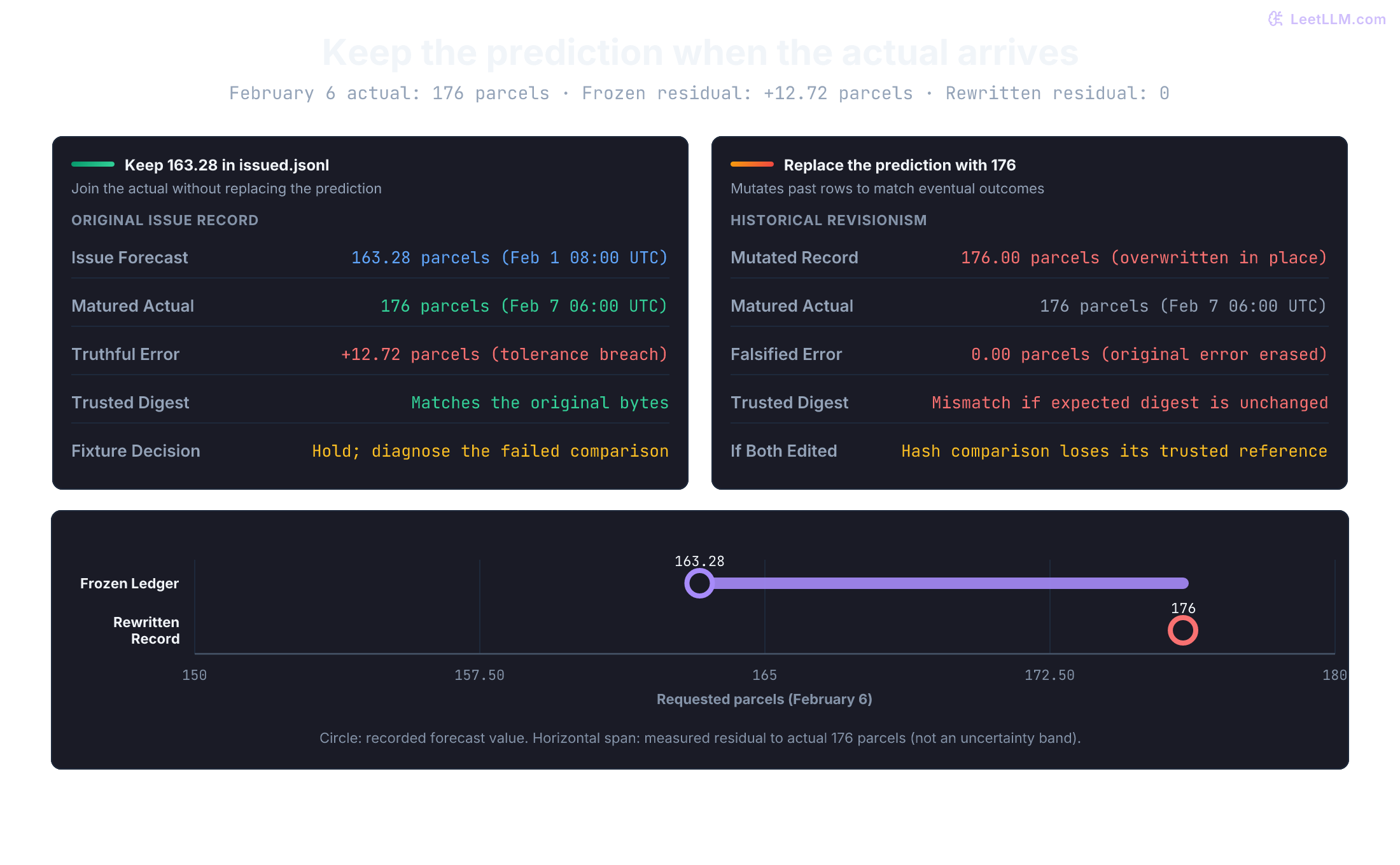
For operational use, retain authorized issue records and their independently protected receipts in storage with appropriate access and retention controls. Preserve input and plan snapshots, feature code, capacity versions, fitted weights, and provenance. The lab supplies source hashes and weights; it doesn't configure those storage controls or keep a revision history for plans.
Evaluate forecasts and operational alerts separately
Evaluate only final observations whose available_at timestamp is no later than the evaluation timestamp. Missing or provisional counts stay pending; they aren't zero volume and aren't silently counted as perfect forecasts.
Check the same frozen ledger at two evaluation times. On February 8, only five target days have mature counts. On February 16, all fourteen do.
early = evaluate(frozen, counts, as_of=ORIGINS[1])
receipt = evaluate(frozen, counts, as_of=AS_OF)
for name, report in (("early", early), ("complete", receipt)):
    print(name, "mature", report["mature"], "pending", report["pending"],
"complete gate", report["gates"]["complete"])early mature 5 pending 9 complete gate False
complete mature 14 pending 0 complete gate TrueFor mature forecasts, mean absolute error is the average of , where is the actual parcel count and is the issued point forecast. Its unit is parcels, matching the target. This is held-out forecast error, not an in-sample training residual.[3]
The authored peak-cost sum activates only on days with at least 150 actual requests and charges . It ignores overforecasts and every lower-volume day, including a Wednesday above its 140-parcel capacity but below 150. It's a selective forecast diagnostic, not total operating cost or a count of unserved parcels. With no mature labels, MAE and peak cost are undefined (None).
Compute both scores, plus the fraction of actuals inside the diagnostic tolerance .
for key in ("baseline_mae", "candidate_mae", "baseline_peak_units",
            "candidate_peak_units", "range_fraction", "residual_breaches"):
    print(key, round(receipt[key], 3))
print("horizon MAE:", {h: round(v, 3) for h, v in receipt["horizon_mae"].items()})baseline_mae 7.643
candidate_mae 6.254
baseline_peak_units 201.0
candidate_peak_units 142.734
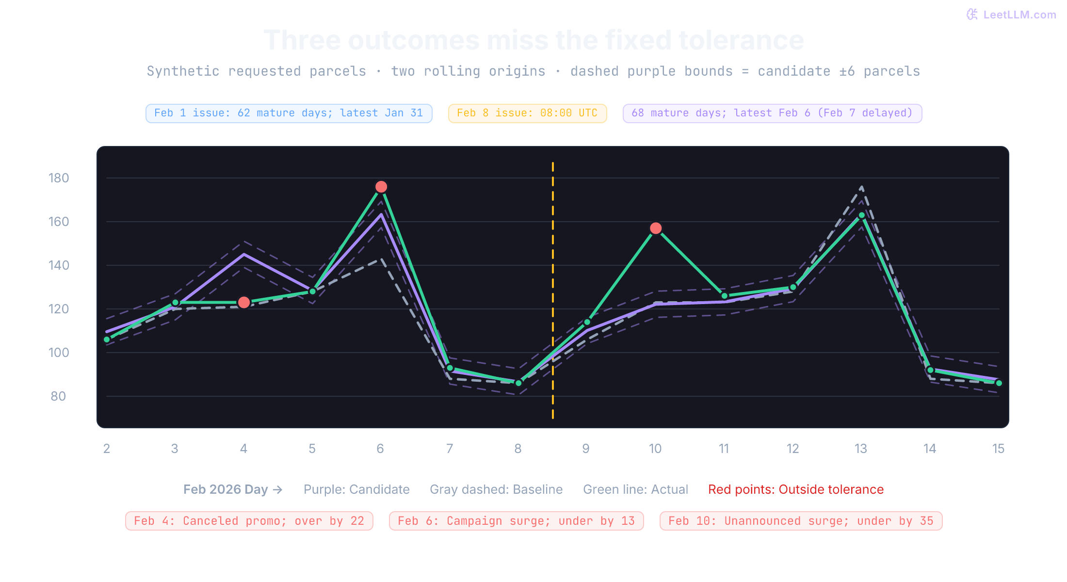
range_fraction 0.786
residual_breaches 3
horizon MAE: {'1': 3.711, '2': 18.428, '3': 12.39, '4': 0.556, '5': 6.634, '6': 0.956, '7': 1.099}The candidate improves MAE from 7.643 to 6.254 parcels and lowers this peak diagnostic from 201 to 142.734 units. Only 11 of 14 actuals fall within tolerance. Horizon 2 has MAE 18.428, driven mostly by February 10's authored surge. Each horizon has two observations. These slices expose cases; they don't establish a stable estimate of future horizon performance. Notice that the largest horizon error isn't at horizon 7.
The six-parcel band is a chosen tolerance, with no stated probability level. A prediction interval instead targets a coverage probability under specified assumptions. Width often grows with horizon, but isn't required to: a mean model's standard interval can have constant width, and a seasonal-naive model's width can stay constant within one season.[6]
For an extension, estimate uncertainty using earlier forecast errors or conditional quantile models, then assess coverage and width on later untouched windows, including relevant horizon and event slices. Estimated quantiles don't automatically guarantee coverage. An observed fraction from fourteen cases isn't proof of calibration. Intervals conditional on a campaign scenario can also miss uncertainty about whether that campaign runs.[5]
Capacity signals need separate tracking. Define the replay proxy as actual > issued capacity. It compares requested volume with the declared schedule; it doesn't observe dock failures, staffing changes, fulfilled volume, or prevented delays. If a planner adds capacity after a warning, retain both the original schedule and the later action to distinguish forecast evaluation from intervention outcomes.
actuals = {str(r.day): r.parcels for r in counts if r.final and r.available_at <= AS_OF}
for row in frozen:
    signal = row.candidate > row.capacity
    overload = actuals[row.target_date] > row.capacity
    if signal or overload:
        print(row.target_date, "signal", signal, "overload", overload)
print("confusion:", receipt["capacity_confusion"])
print("precision:", round(receipt["precision"], 3),
"recall:", round(receipt["recall"], 3))2026-02-04 signal True overload False
2026-02-06 signal True overload True
2026-02-10 signal False overload True
2026-02-13 signal True overload True
confusion: {'tp': 2, 'fp': 1, 'fn': 1, 'tn': 10}
precision: 0.667 recall: 0.667The two campaign Fridays (February 6 and February 13) are true positives. February 4 is a false positive because the planned campaign was canceled. February 10 is a false negative because an unannounced volume spike exceeded capacity without advance notice. Precision is , the fraction of three triggered alerts that correctly predicted an overload. Recall is also , the fraction of three actual overload events successfully caught. Ten true negatives don't enter either denominator.
Notice how February 13 triggered a correct capacity alert without tripping the residual monitor: a forecast can accurately warn of high volume while landing within a few parcels of ground truth. Decouple forward-looking capacity signals from backward-looking residual alerts:
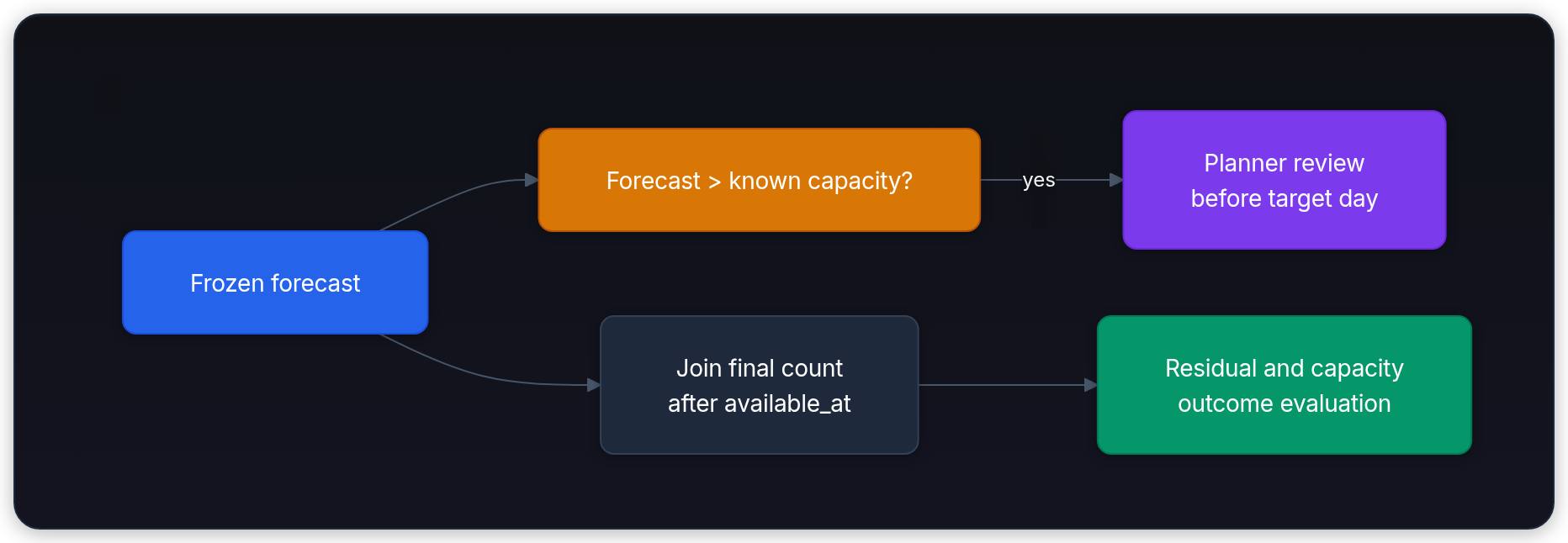
An operational system could route capacity warnings to planners and later residual breaches to model and data owners. The program only calculates these signals. A tolerance breach can reflect changed plans, a missing predictor, an unusual outcome, or bad data; it doesn't diagnose drift or probability miscalibration by itself.
Inspect the comparison before planning a rollout
The local comparison requires both named origins and all seven horizons with mature labels, better MAE and peak cost than baseline, tolerance fraction at least 0.85, and capacity precision and recall at least 0.60. It also requires a nonblank previous-model name. These are fictional acceptance criteria, not industry thresholds. A model name isn't a verified rollback path.
Record comparison_pass separately from operational readiness. Even if every local comparison passes, decision stays hold, reason is synthetic_fixture_only, and live_ready is false. Fitting a contrived dataset doesn't authorize a real planner pilot or deployment.
Display the decision alongside its failed gates.
print("decision:", receipt["decision"])
print("failed:", [name for name, passed in receipt["gates"].items() if not passed])
print("previous:", receipt["previous"])
print("live ready:", receipt["live_ready"], "reason:", receipt["reason"])
print("no-label precision:", evaluate(frozen, [], as_of=AS_OF)["precision"])decision: hold
failed: ['range_fraction']
previous: seasonal-v0
live ready: False reason: synthetic_fixture_only
no-label precision: NoneThe comparison fails because . The residual checks expose the canceled campaign and surge after their counts mature. They don't predict either surprise in advance. Keep the failed comparison, and assess proposed fixes on later data. Widening tolerance on these same outcomes consumes them as development evidence.
A real rollout needs more evidence. After a broader backtest on representative operational data, propose a planner pilot with forecasts alongside the incumbent. Log whether warnings are actionable, redundant, or misleading, and retain actual staffing or booking decisions. Choose the observation period from label delays, sample needs, seasonality, and important events; two quiet weeks can't establish holiday performance. Before shifting decisions, verify a compatible previous model, its data and feature dependencies, and the actual recovery procedure. None of these steps is implemented by the fixture receipt.
Establish retraining triggers and data drift monitoring
Append verified daily counts as they mature, recording both the target date and availability timestamp. Track missing-label rates and data arrival delays separately from model forecast error. A sudden collapse in recorded volume might indicate an upstream tracking tag outage or ETL failure rather than a true drop in consumer demand. Retraining on unverified zeros bakes the pipeline failure directly into model weights.
Specify retraining proposals alongside their observation windows and evidence needs:
- Scheduled fits: this lab refits at two Sunday origins. A weekly expanding or rolling window is one candidate schedule to evaluate.
- Review triggers: a breach fraction above 15% or capacity precision below 60% could be starting examples, not validated alarms. Account for denominator size, label maturity, changed plans, event mix, and repeated monitoring before interpreting a threshold crossing.
Keep each fitted version and its original issue records. Recompute forward comparisons without rewriting prior forecasts, then collect the evidence required by the operational release policy. Lower training error alone doesn't justify replacement. The program doesn't schedule retraining or execute a drift-triggered action.
Verify contract boundaries with deliberate failures
The module's checks mutate unavailable counts, inject a late plan, mark a label provisional, shrink tolerance, and attempt ledger tampering. They also reject malformed flags, nonfinite forecasts, forged IDs, duplicate records, naive timestamps, and a float-valued horizon. Partial windows and a blank previous-model name can't pass completeness and naming checks.
print(failure_checks(counts, plans, frozen))
run_directory.cleanup()Boundary checks passedThe future-count check adds 10,000 to counts unavailable at the first origin. Its seven forecasts remain identical. That tests one specific data path; it doesn't prove that every feature, plan revision, or upstream snapshot is free of leakage.
For a portfolio extension, add timestamped announcement and cancellation versions. Replay the plan state known at each historical origin; an unannounced cancellation mustn't alter an already issued forecast. Then add centers and service tiers with explicit entity keys. Finally, compare quantile-based capacity decisions under a declared underage/overage loss with the OLS forecast. Include booking constraints and actual cost measurements before calling a reduction "freight savings."
Check your diagnosis
Why does the February 8 forecast copy January 25 rather than February 1?
Answer
At the February 1 issue time, that day's final count doesn't exist yet. January 25 is the latest available matching weekday.
Why can the capacity signal be correct even when the residual monitor later fires?
Answer
A forecast can exceed capacity but still underestimate demand. February 6 predicts about 163 against capacity 150, yet actual 176 exceeds the forecast's six-parcel tolerance.
Why doesn't a lower MAE make the receipt pass?
Answer
The gates measure separate requirements. MAE improves, but only 11 of 14 outcomes meet the fixed tolerance, below the declared 85% requirement.