Personalize this lesson
Adapt explanations and teaching visuals to your background and preferred voice.
Model B passed one extra coding task. Is that a durable upgrade, or just a lucky roll of the dice?
A batch solve rate wobbles from run to run, and putting an interval around one model's score still doesn't settle whether it beats its predecessor. In this lesson, we test a coding-assistant upgrade using a suite of six platform-helper tasks: parsing timestamp windows, permission fallbacks, retry budgets, event deduplication, quota rounding, and cache invalidation. Both models face identical prompts and hidden tests that mark each candidate pass or fail. The numbers stay small enough to verify every calculation by hand.
The estimation lesson bounded uncertainty around a single rate; sampling and simulation showed how repeated draws scatter an estimate. Here the target is the difference between two systems. All outcomes below are illustrative fixtures rather than benchmarks of commercial checkpoints. The Python examples rely purely on the standard library.
Before inspecting the task rows, consider a simple question: if five tasks tie and one favors Model B, which rows tell you who actually won?
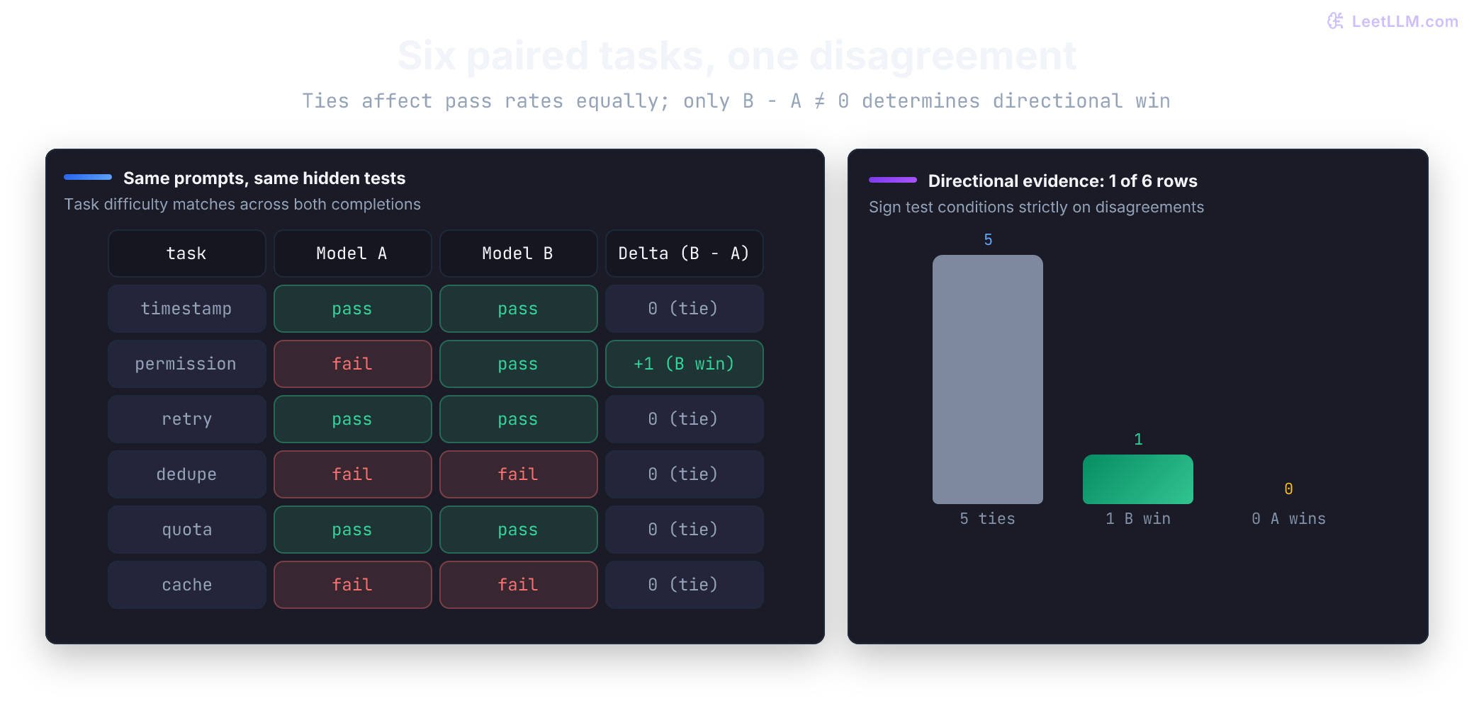
Start with paired pass or fail outcomes
Both models receive the exact same prompt and face the exact same hidden unit tests. That pairing anchors the entire benchmark design. If prompts, test harnesses, or decoding parameters drift between runs, you're no longer measuring a model upgrade; you're measuring environmental noise. Treat each task as a single paired observation rather than two disconnected scores.
The evaluation flow keeps that paired structure visible: one prompt fans out to two completions, which face identical unit tests before computing the task difference.
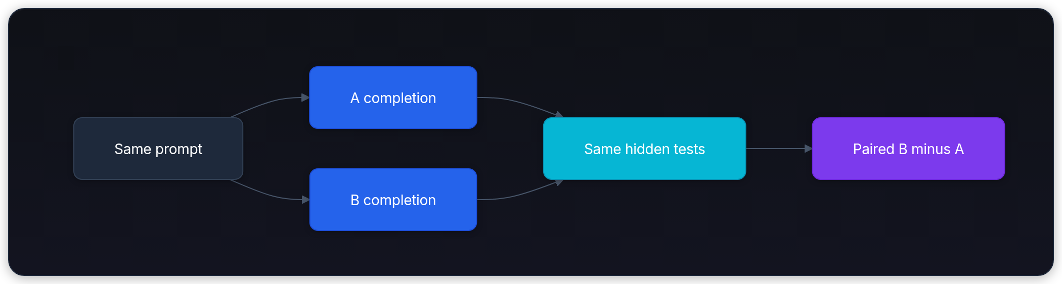
Now inspect the six task outcomes. Look for rows where the two result columns disagree.
| Task | Hidden-test requirement | Model A | Model B |
|---|---|---|---|
| 1 | timestamp range is inclusive | pass | pass |
| 2 | permission fallback preserves denial | fail | pass |
| 3 | retry budget caps at configured limit | pass | pass |
| 4 | event deduplication keeps latest version | fail | fail |
| 5 | quota rounding is deterministic | pass | pass |
| 6 | cache invalidation skips expired keys | fail | fail |
Convert pass to 1 and fail to 0. Model A's pass rate is 3 / 6 = 0.500, Model B's is 4 / 6 = 0.667, and the observed lift is 1 / 6 = 0.167, or 16.7 percentage points.
The next snippet prints those three quantities so you can check the arithmetic against the table.
1model_a = [1, 0, 1, 0, 1, 0]
2model_b = [1, 1, 1, 0, 1, 0]
3
4rate_a = sum(model_a) / len(model_a)
5rate_b = sum(model_b) / len(model_b)
6lift = rate_b - rate_a
7
8print(f"Model A pass@1: {rate_a:.3f}")
9print(f"Model B pass@1: {rate_b:.3f}")
10print(f"observed lift: {lift:+.3f} ({lift * 100:+.1f} percentage points)")1Model A pass@1: 0.500
2Model B pass@1: 0.667
3observed lift: +0.167 (+16.7 percentage points)Looking only at aggregate totals conceals the pairing. Subtract Model A's score from Model B's score on each row:
| Result on one task | Difference B - A | Count |
|---|---|---|
| both pass | 0 | 3 |
| both fail | 0 | 2 |
| B passes, A fails | +1 | 1 |
| A passes, B fails | -1 | 0 |
Only disagreement tasks reveal which model performed better. Ties still shape both overall pass rates and the magnitude of the lift, but not the sign test's conditional win count. That distinction drives the first hypothesis test.
1model_a = [1, 0, 1, 0, 1, 0]
2model_b = [1, 1, 1, 0, 1, 0]
3
4differences = [b - a for a, b in zip(model_a, model_b)]
5b_wins = differences.count(1)
6a_wins = differences.count(-1)
7ties = differences.count(0)
8
9print("paired differences:", differences)
10print(f"B wins={b_wins}, A wins={a_wins}, ties={ties}")
11print("directional evidence comes from disagreements:", b_wins + a_wins)1paired differences: [0, 1, 0, 0, 0, 0]
2B wins=1, A wins=0, ties=5
3directional evidence comes from disagreements: 1A one-task lead exists in this sample. The central question is whether that lead is surprising if both models are equally capable. In other words, how often would a fair comparison produce at least this many wins for Model B?
How surprising is one B win?
Only one row disagreed, and Model B won it. If the two models were equally strong, that row could have fallen either way. The null hypothesis () sets that baseline: on disagreement tasks, Model A and Model B are equally likely to win (). The directional alternative hypothesis () states that Model B wins more frequently ().
Drop the ties and treat each remaining pair as a fair coin toss: Model B wins or Model A wins. That is the exact sign test on disagreements. Dixon and Mood presented this paired sign-test formulation in 1946; the test conditions strictly on the number of disagreements and ignores tied outcomes.[1]
This calculation assumes independent task pairs drawn from the task distribution you want to evaluate. Twenty near-duplicate prompts aren't twenty independent pieces of evidence. For related tasks derived from the same repository or template, use a cluster-level analysis instead of treating each variant as an independent observation.
Our six-task benchmark has one disagreement, and Model B won it. A one-sided p-value for the planned claim "Model B is better" asks:
If both models were equally likely to win a disagreement, how often would random chance hand Model B at least this many wins?
Before running the code, predict what happens with and : can a single win ever be rare when a fair coin has only two outcomes?
If represents the count of disagreements and represents the count of Model B wins, the one-sided right-tail probability is:
The sum counts every outcome at least as favorable to Model B as the observed result. A p-value is this tail probability under the null hypothesis. It isn't the probability that the null hypothesis is true, and it isn't the probability that Model B is better.[2]
With one disagreement, Model B wins it with probability . That result isn't surprising in the slightest.
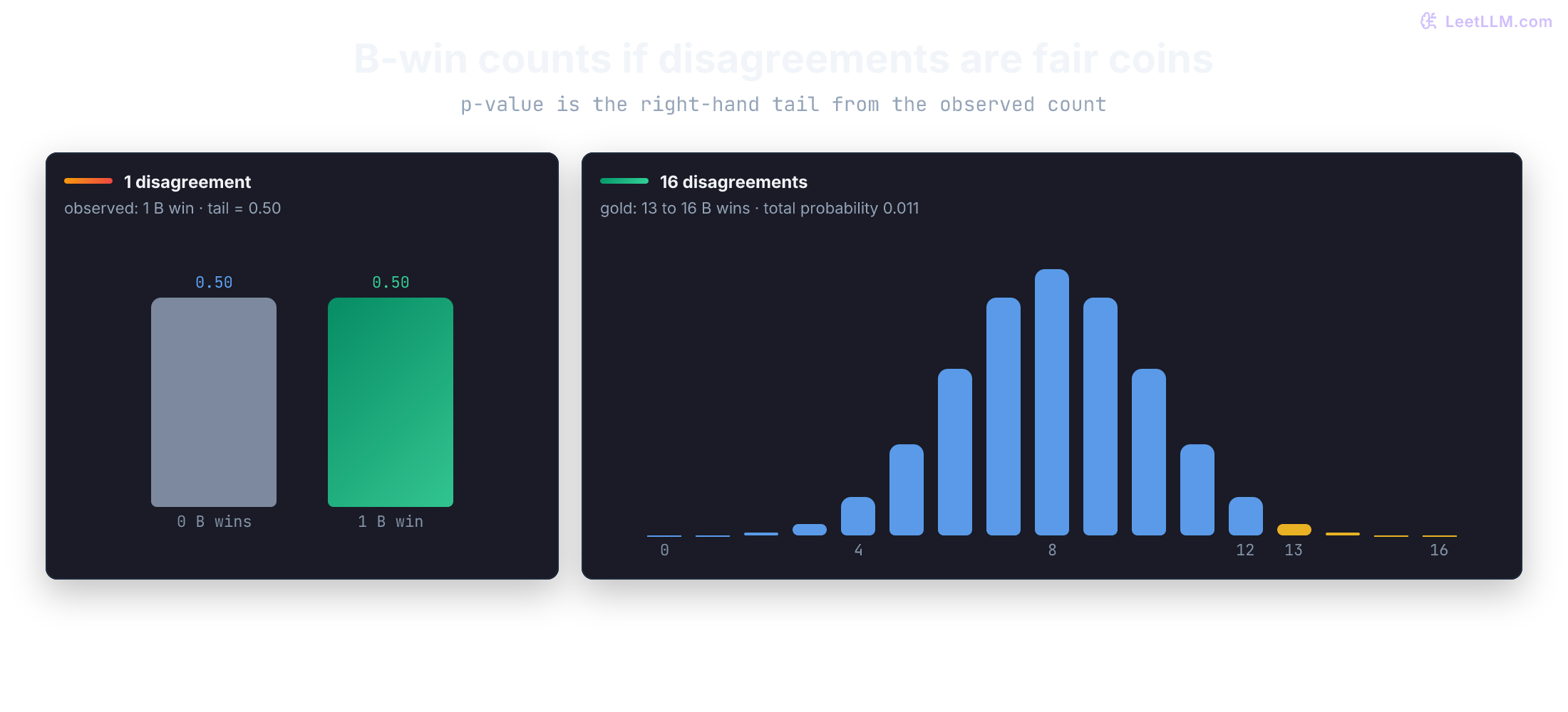
The next function evaluates that exact tail for the one-disagreement fixture and for a larger 13-to-3 outcome:
1from math import comb
2
3def b_wins_one_sided_p_value(b_wins: int, a_wins: int) -> float:
4    if b_wins < 0 or a_wins < 0:
5        raise ValueError("win counts must be nonnegative")
6    disagreements = b_wins + a_wins
7    if disagreements == 0:
8        return 1.0
9    tail_count = sum(comb(disagreements, wins) for wins in range(b_wins, disagreements + 1))
10    return tail_count / (2 ** disagreements)
11
12print(f"one B win, zero A wins: p={b_wins_one_sided_p_value(1, 0):.3f}")
13print(f"thirteen B wins, three A wins: p={b_wins_one_sided_p_value(13, 3):.4f}")1one B win, zero A wins: p=0.500
2thirteen B wins, three A wins: p=0.0106Thirteen wins to three is a completely different story. If you had declared "Model B is better" before seeing the outcomes, that one-sided tail probability is . If you had planned to detect a difference in either direction, the symmetric two-sided binomial test yields about here. Never pick the favorable direction after inspecting who won.[3]
Model B passes four tasks and Model A passes three, but there is only one disagreement. What is the safe conclusion?
Answer
Model B scored higher in this small sample. The single disagreement gives weak evidence for a durable improvement, so you should collect more paired tasks before claiming the model is better.
A p-value answers whether a win is surprising under the null. It doesn't tell you how large the lift is, or whether the test had enough power to detect a real gain.
Type I errors, Type II errors, and statistical power
Every model-review decision is a choice made under uncertainty. In statistical evaluation, two distinct mistakes can occur:
| Reality \ Decision | Retain (Keep Model A) | Reject (Ship Model B) |
|---|---|---|
| is true (B is no better) | Correct retention (Probability: ) | Type I error (, False Positive): Ship phantom gain |
| is true (B is genuinely better) | Type II error (, False Negative): Shelve real improvement | Statistical Power (): Successfully detect lift |
A Type I error () is a false positive: rejecting the null hypothesis when Model B is actually no better (or worse) than Model A. Shipping a false win burns GPU memory, invalidates inference caches, complicates rollbacks, and risks silent user regressions. Setting a significance threshold such as caps the probability of making a Type I error at 5% under the baseline assumption that the null hypothesis is true.
A Type II error () is a false negative: failing to reject the null hypothesis when Model B is genuinely superior. An engineer trains a refined checkpoint that produces a real 3 percentage point lift, but the evaluation suite contains too few tasks to confirm it, so the model gets shelved.
Statistical power () measures the probability of detecting a real improvement of a specific effect size . Power depends directly on four interacting variables:
- Effect size (): Large leaps in model capability are easy to detect; subtle 1% to 2% gains require extensive data.
- Sample size (): Larger task suites provide more chances to observe disagreements and narrow the sampling error.
- Variance (): Noisy prompts obscure the underlying difference.
- Significance threshold (): Stricter false-positive gates (like ) demand stronger evidence, which lowers power unless sample size increases.
In our six-task benchmark with a single disagreement, statistical power against even a massive 20-point lift is practically zero. Because a single fair coin toss has probability , it's mathematically impossible for any one-disagreement result to produce . You could never reject the null on one disagreement, no matter how much better Model B truly is.
Even with 16 disagreements, power against subtle improvements remains modest. When an evaluation yields , that doesn't mean the two models are identical; it often just means the evaluation lacked the statistical power to resolve the difference. Never mistake absence of evidence for evidence of absence.
Looking for a winner changes the test
Suppose the 13-to-3 result was the best of twenty prompt variants tried against Model A. Reporting only its leaves out nineteen opportunities to find a small p-value by pure chance.
A significance level, such as , limits the false-rejection probability for a single, preplanned test under its null. It doesn't guarantee a five-percent chance of error when searching through a catalog of experiments. If twenty independent tests each falsely reject with probability , the probability of observing at least one false rejection across the family is:
One standard safeguard is the Bonferroni correction: for twenty planned comparisons, test each individual comparison at . This adjustment bounds the family-wise error rate even when tests are dependent, provided each p-value is valid. Our result doesn't clear that bar. Bonferroni can be conservative, but the core discipline is to account for all comparisons searched, not just the winner.[4]
Repeatedly inspecting the same benchmark and halting execution the moment is another form of hidden search. Fix the sample size and analysis protocol in advance, or use sequential testing methods designed for continuous monitoring. If an evaluation suite guided prompt or hyperparameter selection, validate the chosen checkpoint on an untouched holdout benchmark. A low p-value isn't a replacement for clean data splits.[2]
Why paired evaluations crush variance
Why do rigorous LLM benchmarks insist on paired evaluations rather than testing Model A on one set of prompts and Model B on another? The mathematical explanation rests on prompt difficulty covariance.
Let represent Model A's pass/fail outcome on task , and let represent Model B's outcome.
If you test Model A on independent prompts and Model B on a separate, unpaired batch of prompts, the variance of the estimated difference between the two sample means is the sum of their individual variances:
In code generation, prompt difficulty varies across an enormous range. Writing an inclusive timestamp filter is straightforward for modern models (roughly a 95% solve rate), while resolving concurrency race conditions or subtle cache invalidations is brutally difficult (often below a 10% solve rate).
When both models attempt the exact same prompt, they share that prompt's difficulty. If task is trivial, both models pass; if task is exceptionally hard, both models fail. Because prompt difficulty affects both models simultaneously, and exhibit strong positive correlation (, typically with correlation ).
In a paired design, the estimator is the sample mean of the row-by-row differences :
The covariance term directly subtracts out the between-prompt variance.
Consider concrete numbers for a benchmark of tasks. Suppose each model has individual pass variance (corresponding to a 50% baseline pass rate), and the prompt difficulty correlation is , giving .
In an unpaired test, the variance is:
The standard error is (11.2 percentage points). An approximate 95% margin of error () spans percentage points. A genuine +7.5 point lift gets lost inside a wide interval.
In a paired test, the covariance term activates:
The variance drops by a factor of 5. The standard error shrinks to (5.0 percentage points), narrowing the 95% error margin to percentage points ().
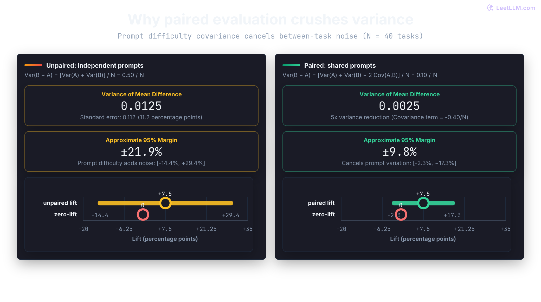
Pairing filters out prompt-to-prompt noise. It gives 40 paired tasks the statistical resolving power of 200 unpaired tasks.
An interval for B minus A
A confidence interval should target the quantity behind the decision. If the question is "How much better is Model B than Model A on this task suite?", build an interval around the paired lift .
Comparing two separate pass-rate intervals can hide the pairing. The evaluation report needs a single interval for the row-by-row difference.
The 95% label describes the intended long-run coverage of the interval procedure over repeated experiments. It doesn't mean this specific realized interval has a 95% probability of containing the true parameter. Classical textbook formulas (such as the Wald interval ) fail on small or discrete benchmarks: they assume symmetric normal sampling distributions, can generate impossible bounds outside , and deliver poor coverage when success rates approach the boundaries.[5]
In the estimation chapter, bootstrap resampling placed an interval around a single metric by drawing observations with replacement.[6] Here the unit of resampling is the paired task row: keep Model A's outcome beside Model B's outcome, then recompute the mean difference. The percentile bootstrap interval takes the 2.5th and 97.5th percentiles of those resampled lifts as its bounds. This task bootstrap reflects sampling variation across a broader population of comparable tasks.[7]
Prediction check: Six tasks help develop intuition but are too few for a stable interval. Consider a slightly larger fixture with 40 paired tasks. Before running the resampler, predict whether a +7.5-point lift from only 13 disagreements will remain strictly positive:
| Paired outcome | Tasks |
|---|---|
| both pass | 17 |
| both fail | 10 |
| B passes, A fails | 8 |
| A passes, B fails | 5 |
The observed lift is , or percentage points. Bootstrap the paired differences to inspect how unstable that lift remains. The next cell resamples complete paired differences and reports the percentile interval.
1from random import Random
2
3differences = [0] * 27 + [1] * 8 + [-1] * 5
4rng = Random(7)
5n = len(differences)
6bootstrap_lifts = [
7    sum(rng.choice(differences) for _ in range(n)) / n
8    for _ in range(20_000)
9]
10
11def quantile(values: list[float], q: float) -> float:
12    ordered = sorted(values)
13    pos = (len(ordered) - 1) * q
14    lo = int(pos)
15    hi = min(lo + 1, len(ordered) - 1)
16    frac = pos - lo
17    return ordered[lo] * (1 - frac) + ordered[hi] * frac
18
19low = quantile(bootstrap_lifts, 0.025)
20high = quantile(bootstrap_lifts, 0.975)
21observed = sum(differences) / n
22at_or_below_zero = sum(lift <= 0 for lift in bootstrap_lifts) / len(bootstrap_lifts)
23
24print(f"observed paired lift: {observed * 100:+.1f} percentage points")
25print(f"approximate 95% bootstrap interval: {low * 100:+.1f} to {high * 100:+.1f} points")
26print("interval includes zero:", low <= 0 <= high)
27print(f"share of resamples with lift <= 0: {at_or_below_zero:.0%}")1observed paired lift: +7.5 percentage points
2approximate 95% bootstrap interval: -10.0 to +25.0 points
3interval includes zero: True
4share of resamples with lift <= 0: 24%Resampling the differences array is equivalent to resampling complete rows for this binary example because each row contributes one difference. With richer multi-metric evals, keep the full row together so the analysis preserves the pairing. The task row, not an isolated model score, remains the fundamental unit of resampling.
The printed 24% is a fraction of bootstrap resamples, not a p-value and not a Bayesian posterior probability that Model B is worse. These resamples center around the observed sample lift; they weren't generated under the zero-lift null hypothesis.
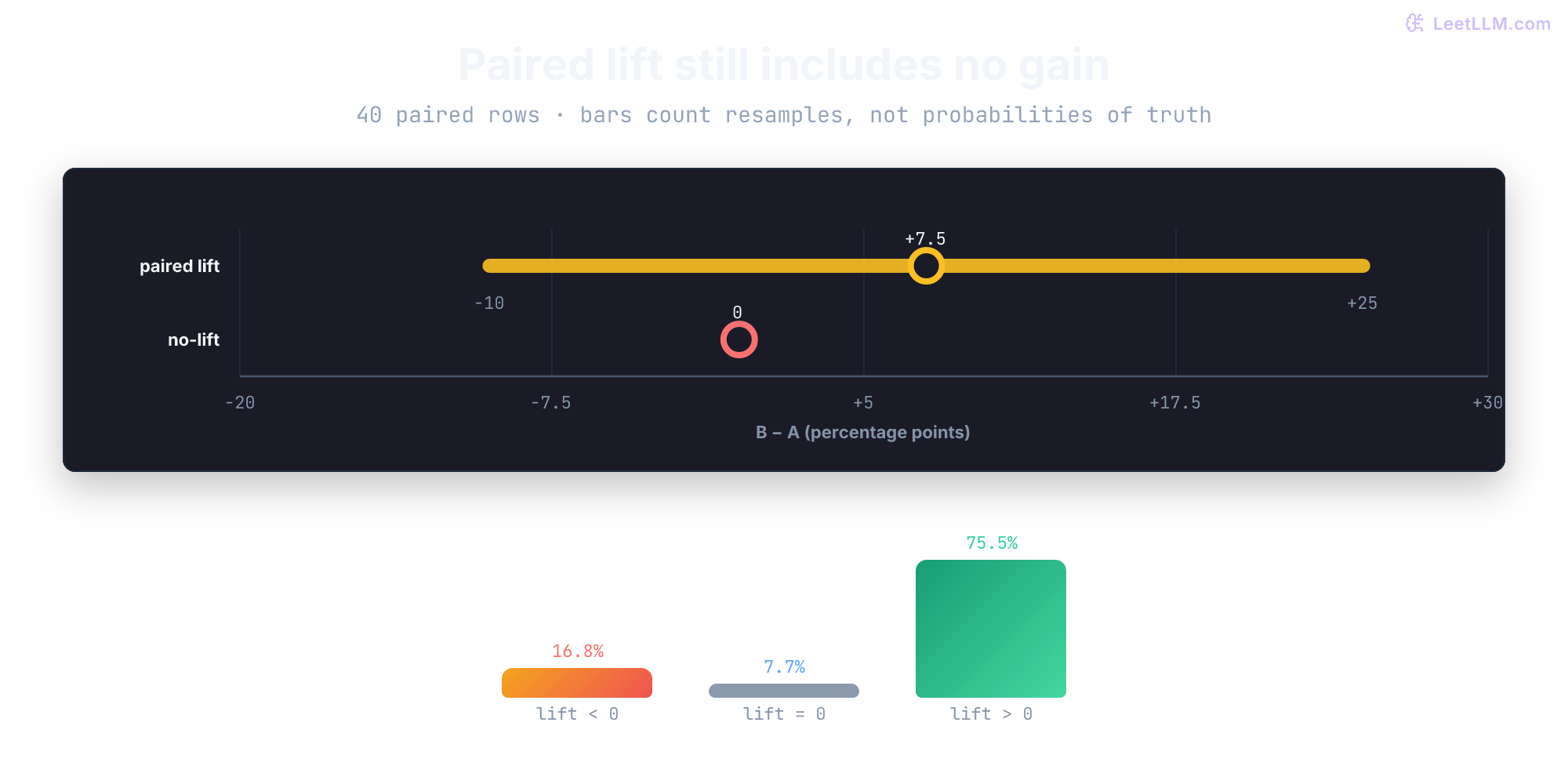
Bootstrap intervals are approximate, especially with small or discrete samples. For instance, resampling six observed ties produces only zero lifts and a [0, 0] interval, even though six ties don't prove the models are identical on future tasks. Running more bootstrap iterations can't conjure missing evidence out of thin air. For our 40-task fixture, the actionable conclusion is: "Model B gained 7.5 points in this paired sample, but the approximate interval spans losses as well as gains."
Set a minimum useful lift threshold before examining results. If deploying Model B requires at least two percentage points of improvement to justify higher hosting costs, an interval of [+1, +14] points excludes zero but doesn't establish the required threshold. The next function formalizes those decisions:
1def comparison_claim(
2    observed_lift: float,
3    interval: tuple[float, float],
4    minimum_useful_lift: float = 0.02,
5) -> str:
6    low, high = interval
7    if low > high or minimum_useful_lift < 0:
8        raise ValueError("require ordered endpoints and a nonnegative useful lift")
9    if low > minimum_useful_lift:
10        return f"clears useful-lift threshold: estimated lift {observed_lift:+.3f}"
11    if low > 0:
12        return f"positive lift, useful size not established: estimate {observed_lift:+.3f}"
13    if high < 0:
14        return f"evidence of regression: estimated lift {observed_lift:+.3f}"
15    return f"inconclusive: estimated lift {observed_lift:+.3f}, interval includes zero"
16
17print(comparison_claim(0.075, (-0.100, 0.250)))
18print(comparison_claim(0.075, (0.010, 0.140)))
19print(comparison_claim(0.075, (0.030, 0.120)))1inconclusive: estimated lift +0.075, interval includes zero
2positive lift, useful size not established: estimate +0.075
3clears useful-lift threshold: estimated lift +0.075So far each task evaluated a single completion from each model. Coding evaluations often permit several candidate attempts. That measures a different capability, and it demands its own evaluation protocol.
pass@k measures attempts
A coding assistant can generate multiple candidate functions, allowing an automated test harness to verify whether at least one candidate passes hidden tests. That is the capability measured by pass@k in functional code-generation benchmarks like HumanEval.[8] The metric fixes a budget of candidate attempts per task. An alternative completion may solve a task that the model's first attempt missed.
HumanEval comprises 164 handwritten Python coding problems with an average of 7.7 unit tests each. In that paper, the authors generated samples per task () and reported up to . Those parameters reflect their specific experimental design, not a rigid requirement. The estimator below works for any predeclared that you run.
Consider this illustrative sample of three platform-helper tasks with three completions each. Follow the retry-state row: only the third candidate passes.
| Task | Attempt 1 | Attempt 2 | Attempt 3 | first_attempt_hit | any_of_3_hit |
|---|---|---|---|---|---|
| parse timestamp window | pass | fail | fail | 1 | 1 |
| retry-state fallback | fail | fail | pass | 0 | 1 |
| quota split rounding | fail | fail | fail | 0 | 0 |
first_attempt_hit records whether Attempt 1 passed. any_of_3_hit records whether any of the three completions passed. Extra attempts discover additional solutions. These realized trials illustrate the underlying concept; a HumanEval-style harness evaluates all sampled candidates to compute an unbiased estimate.
Count each task once in both perspectives:
1attempts = [
2    [1, 0, 0],
3    [0, 0, 1],
4    [0, 0, 0],
5]
6
7first_attempt_hit = sum(row[0] for row in attempts) / len(attempts)
8any_of_3_hit = sum(any(row[:3]) for row in attempts) / len(attempts)
9
10print(f"first_attempt_hit: {first_attempt_hit:.3f}")
11print(f"any_of_3_hit: {any_of_3_hit:.3f}")
12print("extra solved tasks from extra attempts:", int((any_of_3_hit - first_attempt_hit) * len(attempts)))1first_attempt_hit: 0.333
2any_of_3_hit: 0.667
3extra solved tasks from extra attempts: 1The ordered table answered a product question about a known first completion. For reporting standard HumanEval metrics, treat the candidates as an unordered pool and evaluate the combinatorial estimator on the count of correct completions. For the same three tasks with samples each, the correct counts are . The unbiased pass@1 score is the mean of :
When , the combinatorial formula simplifies to , regardless of which completion was generated first. When , the combinatorial estimator equals the any_of_3_hit column. These aren't conflicting definitions: one is a single realized draw, while the estimator computes the expected value over all possible subsets drawn from the generated pool.
Keep two budgets distinct: specifies the operational attempt budget being evaluated; is the number of samples drawn to estimate that metric. You can estimate pass@1 using 200 samples without giving the end product 200 attempts.
When a task has n=10 candidates and c=2 correct, what is HumanEval-style pass@1?
Answer
0.2. For k=1 the combinatorial estimator is c/n. It doesn't depend on which of the ten samples came first in generation order.
Publish , the sample pool size , the decoding parameters, and the test suites used to verify functional correctness. A higher score under a larger candidate budget doesn't imply stronger single-completion performance. Chen and colleagues also observed that higher sampling temperature often benefits larger , because more diverse candidates increase the chance that at least one completion solves the problem.[8]
Derive the HumanEval estimator by hand
Suppose the assistant generates candidate implementations for a function, and hidden tests accept of them. You want to compute the expected pass@5 score if you pick five candidates from that pool. Before calculating, predict which event is easier to count: at least one candidate passing, or all five candidates failing?
Counting successful subsets directly is tedious. Count the failure case instead. The event "at least one candidate passes" is the complement of "all five candidates fail":
- There are failing candidates.
- There are total ways to pick five candidates from the pool.
- There are ways to pick five candidates that all fail.
- The probability that at least one candidate passes is .
In general notation:
The target parameter is generative: the probability that at least one of independent model completions succeeds, written for an unknown per-token solve probability . The combinatorial formula is an unbiased minimum-variance estimator (a U-statistic) of that generative quantity. It calculates the exact fraction of -sized subsets of the completions that contain at least one passing solution. The HumanEval protocol samples and reports this combinatorial estimator rather than a naive plug-in.[8]
Here i.i.d. signifies independent draws from the same decoding distribution for this task. Fix in advance and don't discard duplicate completions: identical outputs still carry probability mass. Halting early after the first passing completion, deduplicating outputs, or feeding test errors back into subsequent attempts alters the experimental distribution. A multi-turn agent that inspects error traces requires an evaluation of that complete iterative harness, not this single-turn formula.
Hidden tests serve as an evaluation oracle: pass@k credits a candidate pool whenever it contains a passing solution. It doesn't assess whether an unguided production system, without access to hidden unit tests, can pick out that passing candidate. Evaluate your reranker or selection model separately if the product must return a single answer.
The next snippet verifies the hand calculation with comb:
1from math import comb
2
3n = 10
4c = 2
5k = 5
6all_groups = comb(n, k)
7all_failing_groups = comb(n - c, k)
8score = 1 - all_failing_groups / all_groups
9
10print("all groups:", all_groups)
11print("all-failing groups:", all_failing_groups)
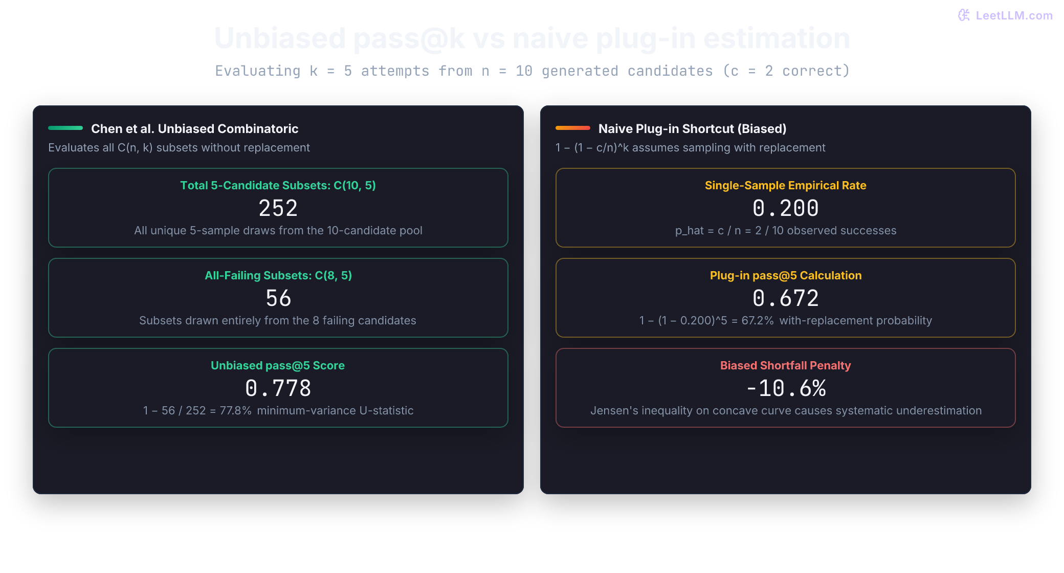
12print(f"pass@5: {score:.3f}")1all groups: 252
2all-failing groups: 56
3pass@5: 0.778How the naive plug-in underestimates pass@k
A tempting shortcut calculates the empirical success rate and substitutes it into the generative formula:
where is the observed single-sample pass rate. Chen and colleagues demonstrated that is a biased underestimate of the generative pass@k probability .[8]
Two distinct mathematical principles explain this shortfall:
- Jensen's inequality on concave functions: Consider the function . For and , the second derivative with respect to is strictly negative: Because is strictly concave, Jensen's inequality guarantees that the expected value of the plug-in estimator is strictly smaller than the true function evaluated at the mean: Plugging a noisy empirical proportion into a concave curve inevitably pushes the estimate downward.
- Sampling with replacement versus without replacement: The plug-in expression represents drawing samples with replacement from the finite pool of completions. Each draw assumes an unchanged failure rate of . But in an actual without-replacement draw, pulling a failing completion removes that failure from the denominator. The proportion of successes among the remaining candidates rises from to . Drawing without replacement depletes the failure pool, making a success more probable on subsequent picks.
For and , the naive plug-in is strictly smaller than the unbiased combinatorial estimate on the same .
For , , and , compare both calculations directly:
1p_hat = c / n
2naive_score = 1.0 - (1.0 - p_hat) ** k
3unbiased_score = score  # From previous cell: 1 - comb(8, 5) / comb(10, 5)
4
5shortfall = unbiased_score - naive_score
6print(f"Plug-in pass@5 1-(1-c/n)^k:            {naive_score:.4f}")
7print(f"Unbiased combinatorial pass@5:         {unbiased_score:.4f}")
8print(f"Plug-in shortfall vs unbiased estimate: {shortfall:.4f}")
9
10assert abs(naive_score - 0.67232) < 1e-51Plug-in pass@5 1-(1-c/n)^k: 0.6723
2Unbiased combinatorial pass@5: 0.7778
3Plug-in shortfall vs unbiased estimate: 0.1055Two boundary checks confirm the logic:
- When , no selected group can pass.
- When fewer than failures exist (), every -sized group contains at least one passing candidate.
For larger , assembling gigantic combinations can trigger floating-point overflow. The HumanEval paper provides an equivalent product formulation that stays numerically well-behaved:[8]
It evaluates the failure probability factor by factor, avoiding factorials of large numbers.
1from math import prod
2
3def pass_at_k(n: int, c: int, k: int) -> float:
4    if n <= 0 or not 0 <= c <= n or not 1 <= k <= n:
5        raise ValueError("require n > 0, 0 <= c <= n, and 1 <= k <= n")
6    if n - c < k:
7        return 1.0
8    failure_probability = prod(1.0 - k / i for i in range(n - c + 1, n + 1))
9    return 1.0 - failure_probability
10
11print(f"n=10, c=2, k=1: {pass_at_k(10, 2, 1):.3f}")
12print(f"n=10, c=2, k=5: {pass_at_k(10, 2, 5):.3f}")
13print(f"no passing candidates: {pass_at_k(10, 0, 5):.3f}")
14print(f"not enough failures: {pass_at_k(10, 8, 5):.3f}")
15
16try:
17    pass_at_k(10, 11, 5)
18except ValueError as error:
19 print(error)1n=10, c=2, k=1: 0.200
2n=10, c=2, k=5: 0.778
3no passing candidates: 0.000
4not enough failures: 1.000
5require n > 0, 0 <= c <= n, and 1 <= k <= nAverage pass@k across tasks
A benchmark score macro-averages task-level results. A complex permission-verification function counts as one task; it shouldn't be drowned out by hundreds of completions from an easy string helper. The estimator runs per task before the benchmark computes its overall mean.
Suppose four tasks each produce candidates, with the following counts of correct completions:
1[0, 1, 2, 4]Compute each task's estimate first, then average those four estimates. A task with zero passing completions contributes zero across every value of .
1correct_counts = [0, 1, 2, 4]
2for k in (1, 3, 5):
3    task_scores = [pass_at_k(10, correct, k) for correct in correct_counts]
4    mean_score = sum(task_scores) / len(task_scores)
5 print(f"pass@{k}: {mean_score:.3f} per-task={[round(score, 3) for score in task_scores]}")1pass@1: 0.175 per-task=[0.0, 0.1, 0.2, 0.4]
2pass@3: 0.417 per-task=[0.0, 0.3, 0.533, 0.833]
3pass@5: 0.563 per-task=[0.0, 0.5, 0.778, 0.976]Notice that pass@5 climbs to while pass@1 sits at . That extra search capacity helps if your production product can verify multiple candidates. It doesn't indicate that single-completion quality improved. The metric grew because the attempt budget expanded, not because the underlying tasks became easier.
Changed protocols create fake wins
To compare models fairly under a fixed sampling policy, keep the task suite, unit tests, candidate budget , and decoding rules matched. Record token cutoffs, execution timeouts, and candidate selection rules. A timeout shouldn't quietly vanish from the denominator.
Record as well, but don't confuse it with . Two independently sampled pools with different predeclared estimate the same underlying pass@k; their precision differs. Matching is a convenient balanced setup, not a mathematical necessity for a valid fixed- benchmark. Don't omit challenging tasks simply because they generated fewer completions than requested: finish the protocol or report that the score can't be computed.[9]
A deterministic decoder illustrates the risk. If every generated candidate is identical, extra sampling slots can't uncover an alternative correct solution. When temperature is zero, pass@5 collapses completely to pass@1.
1identical_failed_candidates = [0] * 10
2identical_passing_candidates = [1] * 10
3
4for name, outcomes in [
5    ("same failed candidate", identical_failed_candidates),
6    ("same passing candidate", identical_passing_candidates),
7]:
8    correct = sum(outcomes)
9 print(name, f"pass@1={pass_at_k(10, correct, 1):.1f}", f"pass@5={pass_at_k(10, correct, 5):.1f}")1same failed candidate pass@1=0.0 pass@5=0.0
2same passing candidate pass@1=1.0 pass@5=1.0Serving engines can introduce nondeterminism from external system factors, so record the exact runtime flags. A degenerate deterministic output distribution remains compatible with independent draws: it simply yields the identical completion on every call. Duplicate completions alone don't prove a protocol violation; they remain in and . A larger represents a larger compute expenditure, not an unearned model upgrade.
Another risk is subtler: code that passes basic unit tests can still harbor edge-case bugs or malicious side effects. Unit-test evaluation establishes functional correctness under that specific suite. It doesn't authorize executing untrusted code directly on host infrastructure.
HumanEval's authors executed model completions inside an isolated sandbox for that exact reason.[8] Treat functional correctness testing and execution isolation as separate, indispensable layers.
Build an evaluation report
Pull the pieces together for a model-review scorecard. The 40-task paired fixture evaluates single-attempt lift. A separate four-task pool evaluates Model B's multi-candidate search behavior. Both require reported uncertainty and a documented protocol; the second fixture isn't a direct comparison with Model A.
This self-contained script runs the calculations and reports each fixture alongside its protocol metadata:
1from itertools import product
2from math import prod
3from random import Random
4
5def pass_at_k(n: int, c: int, k: int) -> float:
6    if n <= 0 or not 0 <= c <= n or not 1 <= k <= n:
7        raise ValueError("require n > 0, 0 <= c <= n, and 1 <= k <= n")
8    if n - c < k:
9        return 1.0
10    return 1.0 - prod(1.0 - k / i for i in range(n - c + 1, n + 1))
11
12def quantile(values: list[float], q: float) -> float:
13    ordered = sorted(values)
14    pos = (len(ordered) - 1) * q
15    lo = int(pos)
16    hi = min(lo + 1, len(ordered) - 1)
17    frac = pos - lo
18    return ordered[lo] * (1 - frac) + ordered[hi] * frac
19
20model_a = [1] * 17 + [0] * 10 + [0] * 8 + [1] * 5
21model_b = [1] * 17 + [0] * 10 + [1] * 8 + [0] * 5
22paired_differences = [b - a for a, b in zip(model_a, model_b)]
23paired_lift = sum(paired_differences) / len(paired_differences)
24rng = Random(7)
25lift_resamples = [
26    sum(rng.choice(paired_differences) for _ in paired_differences)
27    / len(paired_differences)
28    for _ in range(20_000)
29]
30lift_lo, lift_hi = quantile(lift_resamples, 0.025), quantile(lift_resamples, 0.975)
31
32correct_counts_b = [0, 1, 2, 4]
33task_scores = [pass_at_k(10, correct, 5) for correct in correct_counts_b]
34pass5 = sum(task_scores) / len(task_scores)
35# Task-level bootstrap of macro pass@k: every with-replacement resample of the
36# four task scores (4^4 = 256), then percentile interval of the resample means.
37# With only four toy tasks the interval is huge; the point is the reporting contract.
38boot_means = [
39    sum(task_scores[i] for i in idxs) / len(task_scores)
40    for idxs in product(range(len(task_scores)), repeat=len(task_scores))
41]
42pass5_lo, pass5_hi = quantile(boot_means, 0.025), quantile(boot_means, 0.975)
43protocol = {
44    "paired_fixture_tasks": len(model_a),
45    "paired_candidates_per_model_per_task": 1,
46    "candidate_pool_fixture_tasks": len(correct_counts_b),
47    "metric": "hidden-test functional correctness",
48    "samples_per_task": 10,
49    "reported_k": 5,
50    "outcomes": "illustrative fixtures, not live generations",
51}
52
53print(f"paired pass@1 lift: {paired_lift * 100:+.1f} percentage points")
54print(f"approximate 95% lift interval: [{lift_lo * 100:+.1f}, {lift_hi * 100:+.1f}] points")
55print(f"Model B pass@5 on candidate pool: {pass5:.3f}")
56print(f"pass@5 95% task-bootstrap interval: [{pass5_lo:.3f}, {pass5_hi:.3f}]")
57for key, value in protocol.items():
58 print(f"{key}: {value}")1paired pass@1 lift: +7.5 percentage points
2approximate 95% lift interval: [-10.0, +25.0] points
3Model B pass@5 on candidate pool: 0.563
4pass@5 95% task-bootstrap interval: [0.194, 0.877]
5paired_fixture_tasks: 40
6paired_candidates_per_model_per_task: 1
7candidate_pool_fixture_tasks: 4
8metric: hidden-test functional correctness
9samples_per_task: 10
10reported_k: 5
11outcomes: illustrative fixtures, not live generationsFor , pass@k is a nonlinear function of task-level completion counts, which is subsequently averaged across tasks. Resampling tasks and recalculating macro pass@k models task-sampling uncertainty. Comparing Model A and Model B at the same requires per-task estimates from both models: resample the paired differences between them, not two disconnected sets of tasks.
With four toy tasks the bootstrap interval is wide, but width alone doesn't guarantee nominal coverage. This demonstrates the calculation rather than providing enough evidence for a launch decision. This task bootstrap holds the generated completions fixed when resampling rows; it doesn't model how an entirely new batch of completions on the same tasks would vary. For grouped benchmark sets, resample independent clusters rather than pretending every prompt is independent.
Before approving a production rollout, verify that your evaluation report contains:
- An interval for the paired lift rather than two disconnected headline numbers
- The macro pass@k point estimate alongside an empirical bootstrap interval
- The planned hypothesis direction chosen before inspecting test results
- The total count of comparisons evaluated and any family-wise error adjustments
- Explicit checkpoint hashes, prompt templates, decoding seeds, and timeout configs
- Sandboxing guarantees and test suite coverage audits
- Latency and cost ceilings for candidate generation in production
Statistical significance and operational value address different questions. Even ironclad statistical proof can't tell you whether a performance gain justifies additional candidate generation, evaluation overhead, execution latency, or security exposure.
Practice: review a benchmark claim
A teammate submits this update: "Model B is better because its pass@5 reached 64%, whereas Model A's pass@1 was 58%."
Write a code review comment addressing three specific issues:
- Request matched attempt budgets , prompt suites, test suites, and decoding settings, while noting the sample size .
- Ask for the paired lift and its confidence interval under that matched protocol.
- Inquire whether the extra generation budget, verification latency, and compute cost are viable for production serving.
A rigorous rewritten claim should read:
Under the same 200 paired platform-helper tasks and a matched
pass@1protocol, Model B's observed pass rate was 2.5 percentage points higher. The paired 95% interval and serving cost guardrails are reported below; the point estimate alone doesn't justify a production swap.pass@5is documented separately because it reflects a larger candidate search budget.
Why is an interval for B - A preferable to comparing two separate intervals here?
Answer
The tasks are paired: both models solve the same prompts under the same tests. An interval for B - A preserves that pairing and directly measures the quantity the decision needs, which is the model lift.
Why can pass@5 be much higher than pass@1 without proving better single-candidate behavior?
Answer
pass@5 permits five candidate attempts per task. It answers whether at least one of five samples passes, while pass@1 evaluates one sample. The added search budget can raise the score.