Reasoning & Test-Time Compute

A familiar on-call trade-off arrives as capacity_math: estimate GPU memory for eight concurrent branches sharing a 4,000-token prompt, each producing 1,000 continuation tokens, while the queue is already busy. One pass is cheap, but it can omit a KV term. Eight candidates may expose the omission, then occupy the cache headroom needed by the next request. The real question isn't “can the model think harder?” It’s “which extra evidence earns its TTFT, memory, and cost?”

State-space models showed one way to keep one live recurrent decode state fixed as context grows; retained checkpoints and branches still add memory. Reasoning models make a different trade: keep working longer, branch, or check an answer when task difficulty makes that useful. The system buys a chance to catch its own plausible mistake before it commits.

For this example, the useful check is arithmetic. With perfect prefix sharing, cache storage covers 4,000 prompt tokens plus eight separate 1,000-token continuations: 12,000 token positions, not 5,000. Without sharing, it covers 40,000. A fluent explanation is not enough to distinguish those answers; a small independent calculator is.

Classic scaling work focused on train-time compute: more parameters, more data, and more pretraining FLOPs (floating-point operations).^{[1]Reference 1Scaling Laws for Neural Language Modelshttps://arxiv.org/abs/2001.08361}

Work from 2024 onward made a second axis hard to ignore. On hard reasoning tasks, extra compute during generation can improve the answer.^{[2]Reference 2Scaling LLM Test-Time Compute Optimally Can Be More Effective Than Scaling Model Parameters.https://arxiv.org/abs/2408.03314[3]Reference 3Learning to reason with LLMshttps://openai.com/index/learning-to-reason-with-llms/} That is test-time compute scaling. OpenAI's o1 launch post and DeepSeek-R1 made the shift visible, while Snell et al. showed in evaluated math settings that a smaller model with a well-chosen inference policy can beat a much larger model answering once.^{[3]Reference 3Learning to reason with LLMshttps://openai.com/index/learning-to-reason-with-llms/[4]Reference 4DeepSeek-R1: Incentivizing Reasoning Capability in LLMs via Reinforcement Learninghttps://arxiv.org/abs/2501.12948[2]Reference 2Scaling LLM Test-Time Compute Optimally Can Be More Effective Than Scaling Model Parameters.https://arxiv.org/abs/2408.03314}

Provider APIs expose this choice as an effort or thinking control, with names and supported values that vary by model. A useful production skill follows: measure where another token, branch, or check changes correctness, then stop when its latency and cost outweigh that gain. More thinking isn't automatically better.^{[5]Reference 5Does Thinking More Always Help? Mirage of Test-Time Scaling in Reasoning Modelshttps://arxiv.org/abs/2506.04210[6]Reference 6Reasoning modelshttps://developers.openai.com/api/docs/guides/reasoning}

We’ll use capacity_math throughout. Easy lookups stay single-pass. For this request, extra samples, a verifier, or a longer trace might change the answer, but each option consumes budget. Keep the earlier picture of how transformers predict the next token, then choose among single-pass, best-of-N, and guided search by the evidence each path can add. Routing and token budgets are part of that choice, not cleanup after the algorithm.

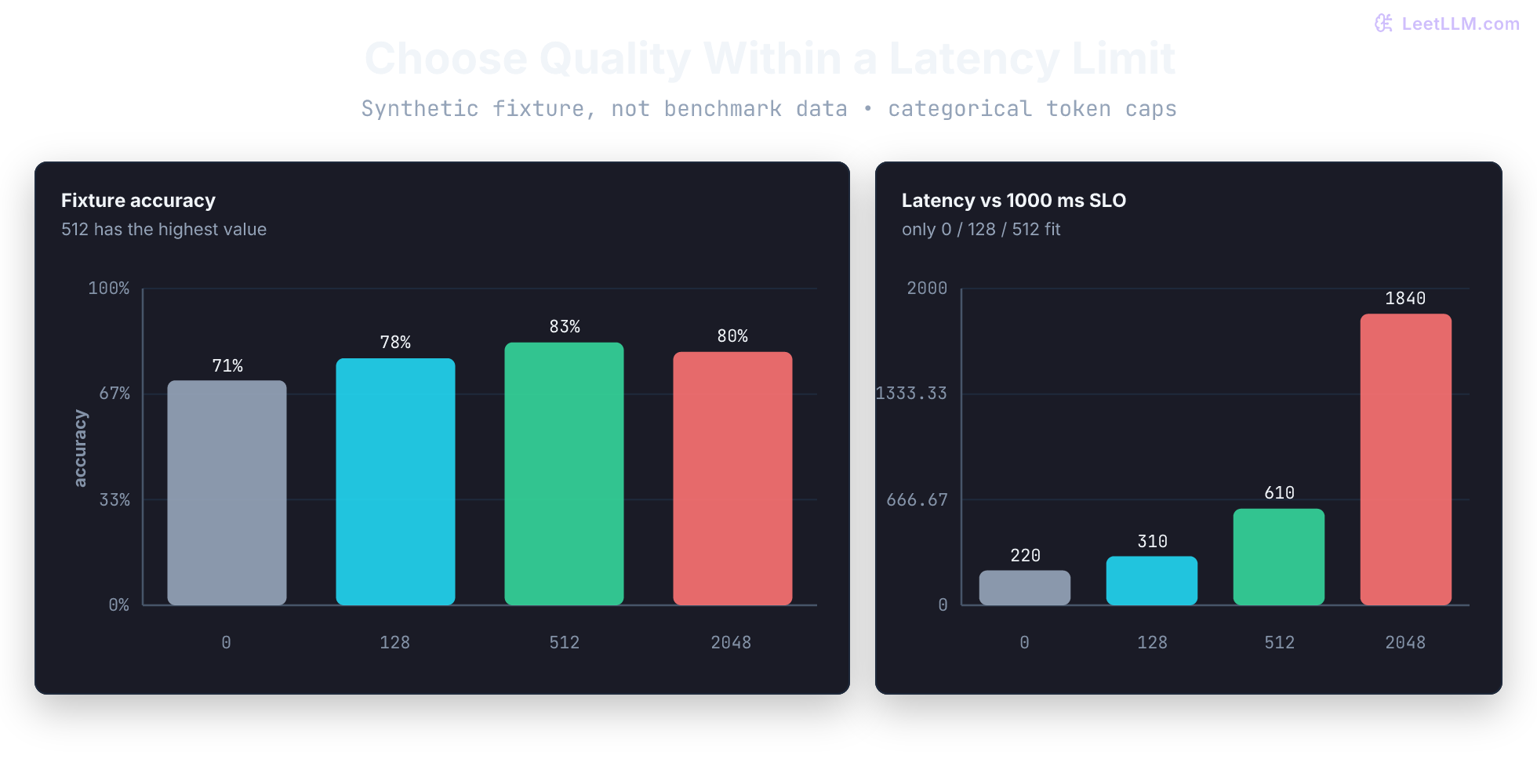
Treat the values as a teaching fixture, not a hardware benchmark. A real sweep records model version, hardware, prompt distribution, sampling policy, verifier, correctness metric, and p50/p99 latency beside each budget.

The two axes of compute scaling

Separate when the bill arrives. Train-time compute is spent before deployment to improve fixed weights. Test-time compute is spent during a live request: trying alternate fixes, checking evidence, and verifying an answer before committing.

Traditional scaling changes model size or training data. Empirical studies fit loss with an approximate power law of compute $C$. Using $N$ for non-embedding dense parameters and $D$ for processed training tokens, the common estimate below follows Kaplan et al.'s roughly $6N$ FLOPs per token for forward plus backward work. Repeated epochs count again in $D$.^{[1]Reference 1Scaling Laws for Neural Language Modelshttps://arxiv.org/abs/2001.08361}

Within the measured regime, that relationship can guide pretraining budgets. The shorthand isn't a physical FLOP count for every architecture: using all stored MoE parameters as $N$ would count experts that a token doesn't execute. It says nothing by itself about which live request deserves a longer rollout.

That live decision adds a second axis, inference compute $C_{\text{infer}}$. A useful model treats accuracy as a function of compute, task shape, policy, and verifier quality:

In an evaluated operating range, more inference compute can improve accuracy with diminishing returns. It can plateau or even reduce accuracy when a trace overthinks, samples remain correlated, or a verifier picks the wrong branch. Compute may arrive as a longer trace, repeated samples, a revision loop, or explicit search with a verifier.^{[2]Reference 2Scaling LLM Test-Time Compute Optimally Can Be More Effective Than Scaling Model Parameters.https://arxiv.org/abs/2408.03314[5]Reference 5Does Thinking More Always Help? Mirage of Test-Time Scaling in Reasoning Modelshttps://arxiv.org/abs/2506.04210}

Snell et al. don't claim one law for every model and benchmark. Their operational result is narrower and more useful: in their math evaluations, a well-allocated inference budget let a smaller model outperform a larger model sampled once.^{[2]Reference 2Scaling LLM Test-Time Compute Optimally Can Be More Effective Than Scaling Model Parameters.https://arxiv.org/abs/2408.03314}

That distinction changes how a system spends compute on a hard prompt:

Traditional approach:     Train bigger → Answer once → Done
Reasoning approach:       Train reasoner → Think longer → Search for best answer

The next cell implements the selection rule on the opening fixture. Real measurements would also need sample counts, uncertainty, and a named latency statistic, such as p99. A point estimate that barely meets a limit is not evidence of reliable compliance.

budgets = [0, 128, 512, 2048]
verified_accuracy = [0.71, 0.78, 0.83, 0.80]
latency_ms = [220, 310, 610, 1840]
latency_limit_ms = 1000

eligible = [
    (accuracy, budget, latency)
    for budget, accuracy, latency in zip(budgets, verified_accuracy, latency_ms, strict=True)
    if latency <= latency_limit_ms
]
if not eligible:
    raise ValueError("no budget meets the latency limit")
# On equal accuracy, prefer less latency, then the smaller budget.
accuracy, budget, latency = max(eligible, key=lambda row: (row[0], -row[2], -row[1]))
print(f"chosen_budget={budget} accuracy={accuracy:.0%} latency_ms={latency}")
print(f"max_budget_is_best={verified_accuracy[-1] == max(verified_accuracy)}")

chosen_budget=512 accuracy=83% latency_ms=610
max_budget_is_best=False

The fixture selects 512. This tests the selection code only. No model, benchmark, or latency measurement ran, and these numbers must not become a production routing policy.

How reasoning models work

Reasoning-oriented training and inference policies allocate additional tokens or branches before returning an answer. You may see decomposition, checks, or revision, but none of those behaviors is guaranteed on every request. Treat them as policies to measure.

Extended chain-of-thought

Reasoning models often generate a long scratchpad or intermediate trace around a final answer. A provider may expose that trace, return a summary, or hide it. Some APIs also interleave non-visible reasoning with visible output or tool calls. For this chapter, the important distinction is operational: can the model or wrapper spend additional inference compute before it commits?

Built-in reasoning also differs from prompted chain-of-thought (CoT)^{[7]Reference 7Chain-of-Thought Prompting Elicits Reasoning in Large Language Models.https://arxiv.org/abs/2201.11903}. Training can shape the policy through Reinforcement Learning (RL), distillation, or both, instead of relying on prompt wording alone. A serving policy can vary the budget by request difficulty, and a trace may backtrack or revise a dead end. Providers can account for and bill that work without exposing raw intermediate tokens.

Current reasoning APIs make the accounting concrete. OpenAI's docs describe reasoning tokens as non-visible output tokens that still consume context budget and count as billed output tokens. They also describe interleaved thinking for some current models, where visible output or tool calls can appear between reasoning steps.^{[6]Reference 6Reasoning modelshttps://developers.openai.com/api/docs/guides/reasoning} The controls below were checked on October 10, 2026; defaults and accepted values belong to the selected model and endpoint.

Reasoning effort is a control for thinking depth, but the contract is model- and endpoint-specific. OpenAI's reasoning.effort accepts a model-dependent subset of none, minimal, low, medium, high, xhigh, and max; lower effort favors speed and lower token use, while higher effort favors more complete reasoning.^{[6]Reference 6Reasoning modelshttps://developers.openai.com/api/docs/guides/reasoning}

Google's current Interactions API uses generation_config.thinking_level and lists supported levels per Gemini model. Its docs represent thoughts and signatures differently in the generateContent API, so a client should follow the selected endpoint's schema instead of copying a knob between APIs.^{[8]Reference 8Gemini thinkinghttps://ai.google.dev/gemini-api/docs/thinking}

Anthropic's docs distinguish adaptive thinking (thinking.type: "adaptive") on newer models from manual budget_tokens on models that support extended thinking. Manual mode is deprecated on Claude 4.6 and rejected on Claude 4.7 and later, while support remains model-specific.^{[9]Reference 9Building with extended thinkinghttps://platform.claude.com/docs/en/build-with-claude/extended-thinking}

Effort is guidance; a token limit is a cutoff. OpenAI Responses uses max_output_tokens for total generated tokens, including reasoning and non-visible formatting, and can return status="incomplete" before any visible text appears.^{[6]Reference 6Reasoning modelshttps://developers.openai.com/api/docs/guides/reasoning} Gemini Interactions likewise counts thoughts toward max_output_tokens; lowering that cap doesn't lower thinking_level, so it can interrupt thinking and leave an empty or truncated answer.^{[8]Reference 8Gemini thinkinghttps://ai.google.dev/gemini-api/docs/thinking} Anthropic adaptive mode uses effort for depth and max_tokens for a hard response limit.^{[9]Reference 9Building with extended thinkinghttps://platform.claude.com/docs/en/build-with-claude/extended-thinking} Don't invent a portable max_reasoning_tokens field or treat a small cap as a guarantee of a useful answer.

Across these systems, higher effort can improve difficult work, but may also increase latency and generated work. Start with clear constraints, tune the supported knob, and evaluate the result instead of assuming a chain-of-thought prompt helps. Count tool calls and scorer work separately from generated tokens when they form part of the policy.

Continuation also has a contract. OpenAI's GPT-5.6 family defaults to making compatible earlier reasoning available with reasoning.context="all_turns"; GPT-6.1 Sol also supports that setting. Inspect the effective reasoning.context on the response rather than infer a default from a newer model name. Prior response items must actually be available, and reasoning doesn't carry across incompatible model families.^{[6]Reference 6Reasoning modelshttps://developers.openai.com/api/docs/guides/reasoning} Gemini Interactions can manage thoughts/signatures through stored interaction IDs; stateless clients must replay thought blocks unchanged, including required tool-result signatures.^{[8]Reference 8Gemini thinkinghttps://ai.google.dev/gemini-api/docs/thinking} A human-readable summary isn't a replacement for that structured state.

Test-time compute can mean a longer single trace or multiple sampled traces. OpenAI's o1 launch post reported one benchmark example on AIME 2024, a math competition: accuracy rose from one sample to consensus over 64 samples, then to learned reranking over 1000 samples.^{[3]Reference 3Learning to reason with LLMshttps://openai.com/index/learning-to-reason-with-llms/} Keep the scope attached to the number. That result belongs to one evaluation, not a promise for another task, model, or selector.

Deliberation and search at inference time

Test-time compute is an umbrella term, not a single algorithm. Some systems sample many complete answers and pick a winner. Some iteratively critique and revise one candidate. Others run explicit search over partial reasoning states using a verifier or reward model. All of these patterns branch from the same idea: spend extra compute to explore, score, and refine before returning an answer.

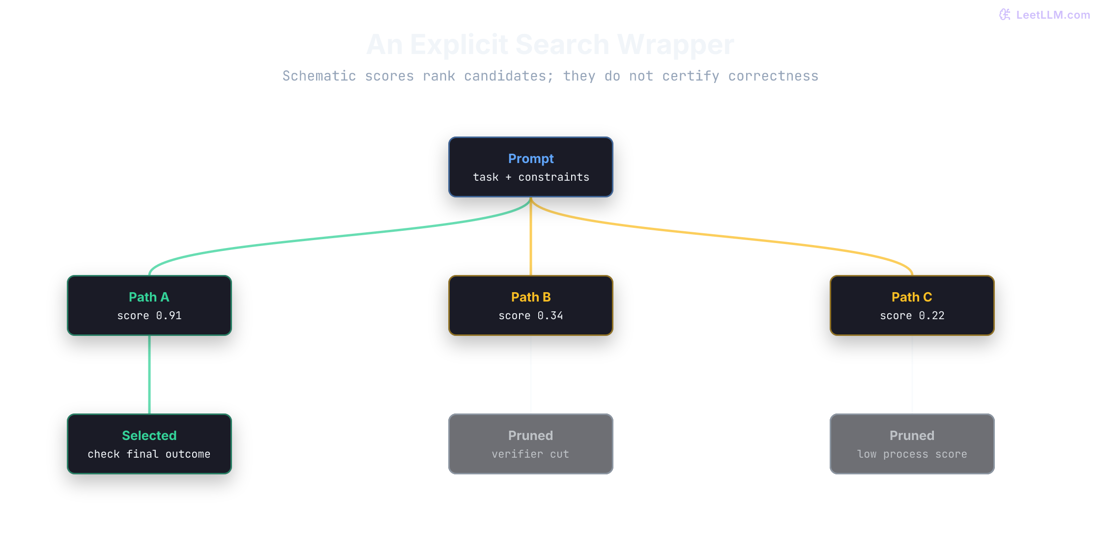
Not every reasoning model literally runs beam search or a PRM at inference time. The shared pattern is optional inference compute allocation. A good routing policy keeps easy requests cheap and assigns more tokens, branches, or verification only where evaluation shows a payoff.

Provider-reported hidden reasoning

Suppose the dashboard shows a short answer but a large output-token count. Some hosted APIs report non-visible reasoning in usage accounting while returning only final text; others interleave visible output or tool calls with non-visible work. OpenAI's reasoning-token documentation describes both patterns.^{[6]Reference 6Reasoning modelshttps://developers.openai.com/api/docs/guides/reasoning} An open-weight deployment, explicit search wrapper, or provider with summarized thinking may expose and account for intermediate work differently, so inspect the actual response schema.

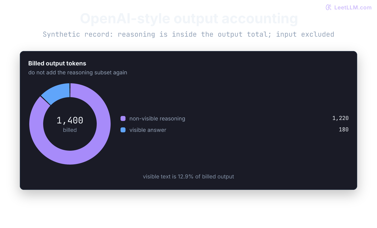
For an API that reports them, non-visible tokens consume context window space and may count toward billing even though users never see them.^{[6]Reference 6Reasoning modelshttps://developers.openai.com/api/docs/guides/reasoning} A transformer runtime that materializes those tokens autoregressively also spends decode work and holds temporary key-value (KV) cache state while generation runs. Exact cache behavior belongs to the provider and engine, not to this accounting shortcut.

The next cell bills the same 180 visible + 1,220 hidden split as the figure, at an illustrative $10 per million output tokens.

usage = {"output_tokens": 1400, "output_tokens_details": {"reasoning_tokens": 1220}}
reasoning_tokens = usage["output_tokens_details"]["reasoning_tokens"]
billed_output_tokens = usage["output_tokens"]
# This fixture has only reasoning and visible text output.
visible_tokens = billed_output_tokens - reasoning_tokens
output_price_per_million = 10.0

cost = billed_output_tokens / 1_000_000 * output_price_per_million
print(f"visible={visible_tokens} billed_output={billed_output_tokens}")
print(f"visible_fraction={visible_tokens / billed_output_tokens:.1%} output_cost=${cost:.4f}")

visible=180 billed_output=1400
visible_fraction=12.9% output_cost=$0.0140

In OpenAI's usage schema, output_tokens already includes output_tokens_details.reasoning_tokens. Adding them again would double-count reasoning.^{[6]Reference 6Reasoning modelshttps://developers.openai.com/api/docs/guides/reasoning} Use the actual provider schema and current prices. This cell calculates output charges only, not the entire request bill or its KV allocation.

That subtraction is specific to this schema and two-part fixture. Gemini Interactions reports total_thought_tokens separately from total_output_tokens; its thinking guide adds the two for generated-token pricing.^{[8]Reference 8Gemini thinkinghttps://ai.google.dev/gemini-api/docs/thinking} Copying one provider's accounting formula into another provider's adapter can undercount or double-count the bill.

Now consider an output cap consumed entirely by reasoning. The following records are fabricated; the cell calls no API. It distinguishes an exhausted response from a completed response that still needs a correctness check.

def next_action(response):
    status = response.get("status")
    if status == "incomplete":
        return "retry_or_escalate"
    if status != "completed":
        return "wait_or_handle_error"
    text = response.get("output_text")
    if not isinstance(text, str) or not text.strip():
        return "no_answer"
    return "check_answer"

records = {
    "hidden-only cutoff": {
        "status": "incomplete",
        "incomplete_details": {"reason": "max_output_tokens"},
        "output_text": "",
        "usage": {"output_tokens": 64,
                  "output_tokens_details": {"reasoning_tokens": 64}},
    },
    "completed guess": {
        "status": "completed", "output_text": "5,000 cached positions",
        "usage": {"output_tokens": 20},
    },
}
for label, record in records.items():
    print(f"{label}: {next_action(record)}, "
          f"billed_output={record['usage']['output_tokens']}")
assert next_action({"status": "completed", "output_text": " "}) == "no_answer"
assert next_action({"status": "in_progress"}) == "wait_or_handle_error"

hidden-only cutoff: retry_or_escalate, billed_output=64
completed guess: check_answer, billed_output=20

The cutoff still costs money. A retry needs a remaining budget and a defined continuation policy; an unconstrained retry loop can multiply the bill. The completed guess is wrong under our opening assumptions, despite having a completed API status.

Test-time compute strategies

When capacity_math is uncertain, extra work can take three forms: parallel candidates, sequential repair, or a branching search that scores partial work. The right pattern follows from what can be checked and how much latency the request can spend.

1. Best-of-N sampling

Sample $N$ candidates for the same prompt, then select one. Best-of-N usually ranks candidates with a scorer; self-consistency instead aggregates their extracted answers, often by plurality vote. A plurality can be wrong. Independently sampled answers can repeat the same learned mistake without being statistically dependent, so diversity alone is not the success criterion.

Best-of-N exposes parallel work, but the engine must have capacity to run it. Eight candidates queued behind one another don't have the latency of eight simultaneous candidates; eight simultaneous candidates can also slow each other under contention. Charge every generated completion and scorer call, even though only one answer returns to the user.

Here is a runnable distinction. The candidates are hand-authored, not model outputs. A trusted calculator checks the stated idealized cache formula. It can't certify real GPU allocation, which also depends on the engine and model architecture.

from collections import Counter

expected_positions = 4000 + 8 * 1000
candidates = [5000, 5000, 12000, 40000]
plurality = Counter(candidates).most_common(1)[0][0]
accepted = [value for value in candidates if type(value) is int and value == expected_positions]
selected = accepted[0] if accepted else None
print(f"plurality={plurality} correct={plurality == expected_positions}")
print(f"verified_selection={selected}")
assert not [value for value in [5000, 40000] if value == expected_positions]

plurality=5000 correct=False
verified_selection=12000

Scaling behavior

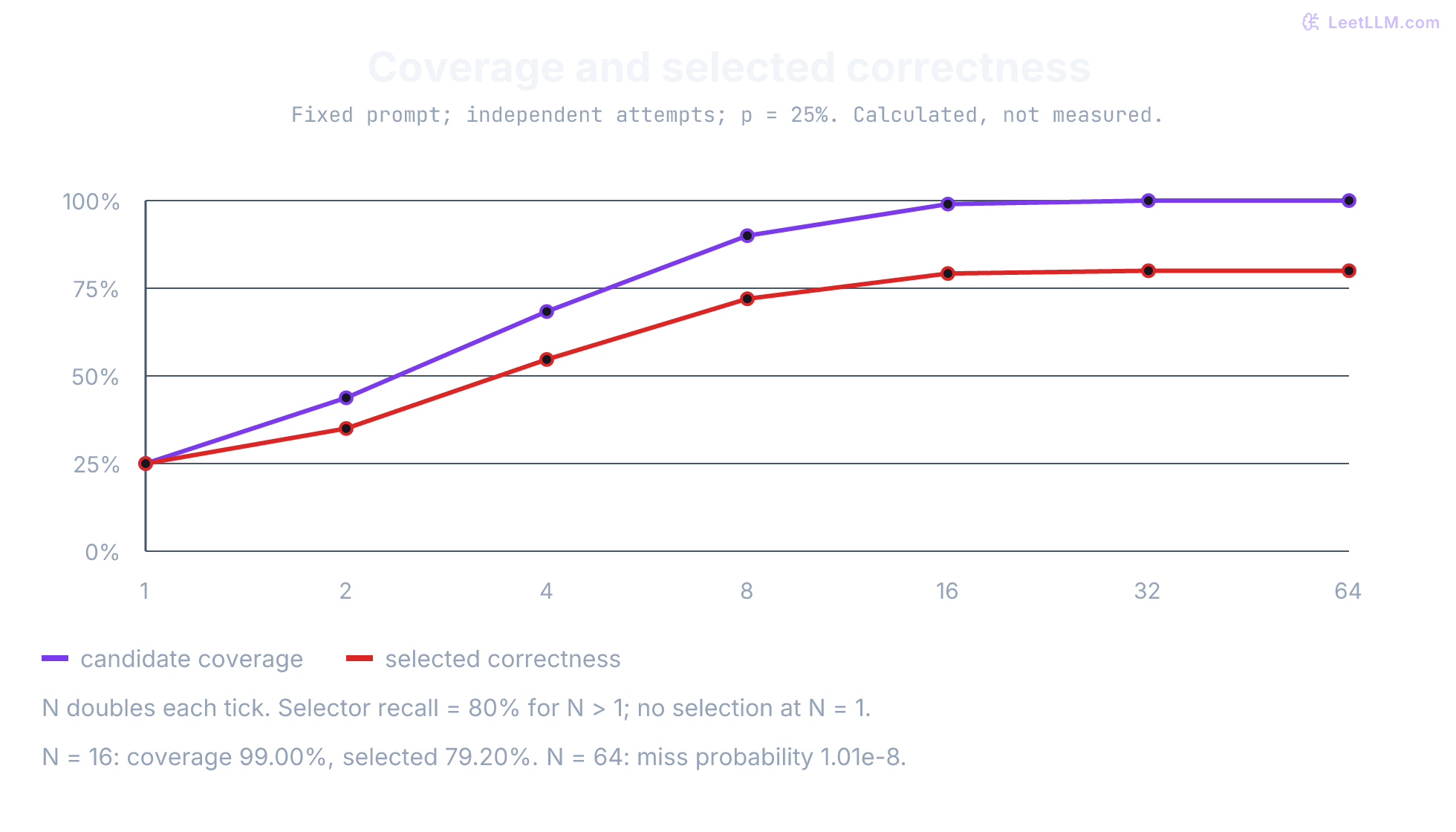
Ask first what an ideal selector would achieve. With an oracle verifier and independent samples, the chance of generating at least one correct answer in $N$ tries follows:

Here $p$ is the success probability for one fixed prompt and sampling policy, with independent, identically distributed attempts. For $p=0.25$, four attempts contain a correct answer with probability $1-(0.75)^4=68.4\%$. That is candidate coverage, not the accuracy of the selected answer. Dependence changes the formula; selection errors can lose an answer already present. Across prompts with different hit rates, average their individual coverage probabilities instead of inserting the dataset-average $p$ into this equation.

import math

def success_probability(p: float, n: int) -> float:
    # This worksheet supports up to a million attempts, not unbounded counts.
    if type(p) not in (int, float) or not 0 <= p <= 1:
        raise ValueError("p must be a finite number in [0, 1]")
    if type(n) is not int or not 1 <= n <= 1_000_000:
        raise ValueError("n must be an integer from 1 to 1,000,000")
    if p == 1:
        return 1.0
    # Avoid losing a tiny p when floating-point subtraction rounds 1-p to 1.
    return -math.expm1(n * math.log1p(-p))

base_hit_rate = 0.25
tokens_per_attempt = 800

for n in [1, 4, 16, 64]:
    success = success_probability(base_hit_rate, n)
    output_tokens = n * tokens_per_attempt
    print(f"N={n:>2} coverage={success:5.1%} miss_probability={(1-base_hit_rate)**n:.2e} output_tokens={output_tokens:>5}")

assert success_probability(0, 4) == 0
assert success_probability(1, 4) == 1
assert math.isclose(success_probability(1e-20, 4), 4e-20, rel_tol=1e-12)
for invalid_p, invalid_n in [(True, 4), ("0.25", 4), (float("nan"), 4),
                             (0.25, True), (0.25, 10**1000)]:
    try:
        success_probability(invalid_p, invalid_n)
    except ValueError:
        pass
    else:
        raise AssertionError("invalid coverage input accepted")

N= 1 coverage=25.0% miss_probability=7.50e-01 output_tokens=  800
N= 4 coverage=68.4% miss_probability=3.16e-01 output_tokens= 3200
N=16 coverage=99.0% miss_probability=1.00e-02 output_tokens=12800
N=64 coverage=100.0% miss_probability=1.01e-08 output_tokens=51200

The rounded 100.0% at $N=64$ is not certainty: the miss probability remains positive. Token cost here grows linearly because every candidate is assumed to have the same length; real lengths vary, and scorer calls add work. The next cell assumes a selector chooses a correct answer 80% of the time conditional on one existing. This constant recall is a teaching assumption, not a property of real selectors.

def selected_success_probability(candidate_success: float, selector_recall: float, n: int) -> float:
    return candidate_success if n == 1 else candidate_success * selector_recall

base_hit_rate = 0.25
selector_recall = 0.80
for n in [1, 4, 16]:
    oracle_success = 1 - (1 - base_hit_rate) ** n
    deployed_success = selected_success_probability(oracle_success, selector_recall, n)
    print(f"N={n:>2} oracle={oracle_success:5.1%} with_selector={deployed_success:5.1%}")

N= 1 oracle=25.0% with_selector=25.0%
N= 4 oracle=68.4% with_selector=54.7%
N=16 oracle=99.0% with_selector=79.2%

The selector is deliberately simple. One candidate has no selection step. Once branches exist, generation and selection become separate failure surfaces: a correct answer can appear and still be discarded.

Real selector recall can change with N. More search also gives a flawed scorer more chances to encounter an answer it overrates. Snell et al. observed verifier exploitation and over-optimization in their search experiments.^{[2]Reference 2Scaling LLM Test-Time Compute Optimally Can Be More Effective Than Scaling Model Parameters.https://arxiv.org/abs/2408.03314} Here is a deterministic counterexample, with hand-authored scores rather than sampled model outputs:

expected_positions = 4000 + 8 * 1000
scored_candidates = [(12000, 0.82), (5000, 0.70), (40000, 0.95)]
for n in (1, 2, 3):
    candidates = scored_candidates[:n]
    selected, score = max(candidates, key=lambda row: row[1])
    coverage = any(answer == expected_positions for answer, _ in candidates)
    print(f"N={n} contains_correct={coverage} selected={selected} "
          f"correct={selected == expected_positions} score={score:.2f}")

N=1 contains_correct=True selected=12000 correct=True score=0.82
N=2 contains_correct=True selected=12000 correct=True score=0.82
N=3 contains_correct=True selected=40000 correct=False score=0.95

Coverage never falls, yet the selected answer becomes wrong. This fixture doesn't estimate a model's probability curve. Evaluate selected correctness with an independent check at each search budget; the search scorer's increasing maximum isn't evidence of improvement.

Train for the test-time policy you plan to use

Training and serving need to agree on what counts as success. Cross-entropy (CE) rewards likelihood of demonstrated target tokens; it doesn't directly optimize correctness or pass@N. For a fixed prompt under independent sampling, raising its true success probability necessarily raises coverage at every N. A dataset average can behave differently: gains on already-easy problems may hide losses on hard ones.

This two-prompt counterexample models a hypothetical change in hit rates, not CE training.

for label, rates in [("before", [0.80, 0.20]), ("after", [0.99, 0.05])]:
    pass_one = sum(rates) / len(rates)
    pass_four = sum(1 - (1 - p) ** 4 for p in rates) / len(rates)
    print(f"{label}: pass@1={pass_one:.1%} pass@4={pass_four:.1%}")

before: pass@1=50.0% pass@4=79.4%
after: pass@1=52.0% pass@4=59.3%

Chen et al. report this mismatch in mathematical reasoning and theorem-proving settings: longer CE training can raise confidence while lowering pass@N, while a confidence-limiting objective better matches later search.^{[10]Reference 10Rethinking Fine-Tuning when Scaling Test-Time Compute: Limiting Confidence Improves Mathematical Reasoninghttps://proceedings.neurips.cc/paper_files/paper/2025/hash/e8f4eae0a41cab67fdead3aa6b77f083-Abstract-Conference.html} CE isn't a failed objective. Evaluate it against the policy you will ship: next-token loss, pass@1, candidate diversity, and pass@N at the actual sample budget.

2. Sequential revision

Now make the work sequential. Draft the capacity_math answer, check it against the KV formula and latency SLO, then repair the weak step. Each pass sees the previous answer, unlike best-of-N's independent attempts.

The loop is draft, check, and regenerate when needed. Preserve the best externally checked candidate: a revision can break a correct answer. A model saying “no errors found” is not an independent verification result. If each revision uses one critique call and one rewrite call, R revisions cost up to 1 + 2R generation calls, plus any separate checks. Those calls are sequential dependencies, not just extra parallel capacity.

The next cell uses synthetic scores to stop after an improvement below 0.01. The round that reveals the plateau has already run and must be charged. A plateau is a budget heuristic, not proof that later revisions can't help.

fixture_scores = [0.61, 0.76, 0.78, 0.781, 0.781]
minimum_gain = 0.01
evaluated_rounds = 1
best_score = fixture_scores[0]

for current in fixture_scores[1:]:
    evaluated_rounds += 1  # We paid for this result before seeing its score.
    gain = current - best_score
    best_score = max(best_score, current)
    if gain < minimum_gain:
        break

print(f"evaluated_rounds={evaluated_rounds} selected_score={best_score:.3f}")
print(f"skipped_rounds={len(fixture_scores) - evaluated_rounds}")

evaluated_rounds=4 selected_score=0.781
skipped_rounds=1

3. Tree search with process reward models

Tree search spends compute before a path is complete. For capacity_math, one branch might multiply KV bytes correctly, another might keep the wrong branch count, and a third might violate the SLO. A process reward model scores each intermediate step, so the controller can prune a bad path before paying for its remaining steps. An outcome score waits for the final answer.

The simplified beam search below starts with one prompt state. Each round proposes several next steps, scores them with the PRM, and keeps the highest-scoring unfinished paths. A branch whose next step starts with Final: moves into a separate completed pool. Search stops when no active branch remains, the budget runs out, or the best completed score bounds every retained unfinished path.

The return value makes completion explicit. It selects the highest-scoring completed chain when one exists. If every branch exhausts the budget without a final answer, it returns the best partial chain with status="incomplete"; the caller can retry, increase the budget, or escalate instead of presenting partial reasoning as an answer. model.generate_step and prm.score_step remain conceptual interfaces here.

def is_final_answer(step: str) -> bool:
    return step.lstrip().lower().startswith("final:") and bool(step.split(":", 1)[1].strip())

def beam_search_with_prm(
    model,
    prm,
    prompt: str,
    beam_width: int = 4,
    branch_factor: int = 4,
    max_steps: int = 20
):
    """Guided tree search using per-step reward scores.

    At most beam_width × branch_factor × max_steps proposals and scores.
    Each proposal may itself require many autoregressive forward passes.
    """
    if any(type(value) is not int or value < 1 for value in (beam_width, branch_factor, max_steps)):
        raise ValueError("beam_width, branch_factor, and max_steps must be positive integers")

    active = [{"steps": [], "score": 1.0, "text": prompt}]
    completed = []

    for _ in range(max_steps):
        candidates = []
        for beam in active:
            # Generate next reasoning step
            new_steps = [
                model.generate_step(beam["text"])
                for _ in range(branch_factor)
            ]

            for new_step in new_steps:
                if not isinstance(new_step, str) or not new_step.strip():
                    raise ValueError("a generated step must be nonempty text")
                # Score each step with the process reward model
                step_score = prm.score_step(
                    prompt, beam["steps"], new_step
                )
                if type(step_score) not in (int, float) or not 0 <= step_score <= 1:
                    raise ValueError("step scores must be finite numbers in [0, 1]")
                candidate = {
                    "steps": beam["steps"] + [new_step],
                    "score": min(beam["score"], step_score),
                    "text": beam["text"] + "\n" + new_step,
                }
                if is_final_answer(new_step):
                    completed.append(candidate)
                else:
                    candidates.append(candidate)

        # Only unfinished branches remain eligible for expansion.
        active = sorted(
            candidates,
            key=lambda candidate: candidate["score"],
            reverse=True,
        )[:beam_width]

        if not active:
            break

        # A descendant's minimum score cannot exceed its parent's score.
        if completed and max(chain["score"] for chain in completed) >= active[0]["score"]:
            break

    if completed:
        best = max(completed, key=lambda candidate: candidate["score"])
        return {**best, "status": "completed"}

    best = max(active, key=lambda candidate: candidate["score"])
    return {**best, "status": "incomplete"}

Completion is a syntax condition here, not correctness: Final: wrong answer is still completed. The controller ranks chains by their minimum step score, a bottleneck heuristic that avoids rewarding length merely for adding positive terms. It isn't a calibrated probability of correctness. Validate the aggregation rule on your task and separately check the final result before calling it verified.

That aggregation also gives a stopping bound: appending a step can only keep or lower a chain's minimum. A completed score of 0.9 therefore cannot be beaten by descendants of retained paths scored at most 0.8. This preserves the winner within this beam's retained search, with ties favoring the existing completed answer. It doesn't recover pruned paths or prove correctness. A last-step score can rise, so the same bound would be invalid for that aggregation rule.

Beam search also tends to collapse onto near-duplicate paths. More capable systems inject diversity, backtrack, or use Monte Carlo Tree Search-style expansion. The tree is easier to write than a verifier that reliably knows which partial step deserves more budget.

The deterministic fixture below exercises both boundaries. In the first run, an unfinished branch reaches a higher score than either final branch, but the selector still returns the best completed answer. In the second run, no branch finishes, so the result is visibly incomplete.

from collections import defaultdict

class ScriptedModel:
    def __init__(self, choices):
        self.choices = choices
        self.calls = defaultdict(int)

    def generate_step(self, text):
        index = self.calls[text]
        self.calls[text] += 1
        return self.choices[text][index]

class ScriptedPRM:
    def __init__(self, scores):
        self.scores = scores

    def score_step(self, prompt, previous_steps, new_step):
        return self.scores[new_step]

model = ScriptedModel({
    "capacity_math": ["keep checking", "Final: early guess"],
    "capacity_math\nkeep checking": ["continue unchecked", "Final: candidate B"],
    "capacity_math\nkeep checking\ncontinue unchecked": [
        "still unfinished A",
        "still unfinished B",
    ],
})
prm = ScriptedPRM({
    "keep checking": 0.9,
    "Final: early guess": 0.7,
    "continue unchecked": 0.9,
    "Final: candidate B": 0.8,
    "still unfinished A": 0.9,
    "still unfinished B": 0.8,
})

selected = beam_search_with_prm(
    model,
    prm,
    "capacity_math",
    beam_width=1,
    branch_factor=2,
    max_steps=3,
)
print(f"selected={selected['steps'][-1]} status={selected['status']}")

unfinished = beam_search_with_prm(
    ScriptedModel({
        "capacity_math": ["keep checking"],
        "capacity_math\nkeep checking": ["still checking"],
    }),
    ScriptedPRM({"keep checking": 0.9, "still checking": 0.8}),
    "capacity_math",
    beam_width=1,
    branch_factor=1,
    max_steps=2,
)
print(f"selected={unfinished['steps'][-1]} status={unfinished['status']}")

wrong = beam_search_with_prm(
    ScriptedModel({"capacity_math": ["Final: 5000"]}),
    ScriptedPRM({"Final: 5000": 0.99}),
    "capacity_math", beam_width=1, branch_factor=1, max_steps=1,
)
print(f"syntactic_status={wrong['status']} "
      f"final_correct={wrong['steps'][-1] == 'Final: 12000'}")

bounded_model = ScriptedModel({
    "capacity_math": ["Final: 12000", "keep checking"],
})
bounded = beam_search_with_prm(
    bounded_model,
    ScriptedPRM({"Final: 12000": 0.9, "keep checking": 0.8}),
    "capacity_math", beam_width=1, branch_factor=2, max_steps=20,
)
assert bounded["steps"] == ["Final: 12000"]
assert sum(bounded_model.calls.values()) == 2
print("bounded winner proposals:", sum(bounded_model.calls.values()))

for invalid_score in (True, "0.8", float("nan"), 10**1000):
    try:
        beam_search_with_prm(
            ScriptedModel({"capacity_math": ["Final: 12000"]}),
            ScriptedPRM({"Final: 12000": invalid_score}),
            "capacity_math", beam_width=1, branch_factor=1, max_steps=1,
        )
    except ValueError:
        pass
    else:
        raise AssertionError("invalid process score accepted")

selected=Final: candidate B status=completed
selected=still checking status=incomplete
syntactic_status=completed final_correct=False
bounded winner proposals: 2

Process reward models vs. outcome reward models

The reward model determines when search gets evidence. If a branch fails only at its final answer, all earlier work is sunk. If partial steps predict failure reliably, the controller can spend the next token on a different branch.

Final scoring and step scoring answer different questions. An ORM asks whether the completed answer works: “the GPU count matches” or “it doesn't.” No intermediate failure location reaches the search controller. A PRM asks about intermediate decisions: “KV formula used,” “branch count held at eight,” “prefix sharing applied.” That denser feedback costs more to build and can discard a good path when wrong. Reliable step scores can still save work by redirecting search early.

Outcome reward models (ORMs)

Outcome Reward Models (ORMs) evaluate a completed trajectory rather than its intermediate steps. The outcome signal may be binary correctness, a probability or scalar score, or a preference-derived comparison. Exact-answer math makes binary grading convenient, but that isn't part of the ORM definition.

Their supervision boundary is relatively simple: labels attach to completed outputs rather than every reasoning step. Verifiable tasks can supply labels automatically; subjective tasks may need learned or human preference signals. During search, though, the ORM has to wait. A generator can make a fatal error in step 1 and produce 100 more steps before the final score rejects the trajectory, so no early branch pruning is available.

How PRMs work

Process Reward Models (PRMs) assign scores at intermediate steps, conditioned on the problem and preceding steps. What the score means depends on its training target. Human validity labels ask whether a step is correct; rollout-based targets can ask whether the current prefix lets a particular continuation policy reach a correct answer. Recoverability and local validity aren't equivalent: a later step can repair an earlier error.^{[11]Reference 11Let's Verify Step by Step.https://arxiv.org/abs/2305.20050[12]Reference 12Math-Shepherd: Verify and Reinforce LLMs Step-by-step without Human Annotationshttps://arxiv.org/abs/2312.08935}

PRMs also need step-level supervision. Lightman et al. trained their strongest PRM with human step labels, while Math-Shepherd estimates whether any sampled completion succeeds (hard target) or the fraction that succeeds (soft target).^{[11]Reference 11Let's Verify Step by Step.https://arxiv.org/abs/2305.20050[12]Reference 12Math-Shepherd: Verify and Reinforce LLMs Step-by-step without Human Annotationshttps://arxiv.org/abs/2312.08935} Those estimates depend on the completer and sample budget. A process score is earlier evidence for keeping or abandoning a branch, not proof that a kept step is correct.

Ask what label an already-wrong step receives if later completions repair it. This fixture declares four completion answers; it doesn't run a completer or train a PRM.

# Current step claims "2 + 2 = 5". Three continuations correct it to 4.
local_step_valid = (2 + 2 == 5)
completion_answers = [4, 5, 4, 4]
successes = [answer == 2 + 2 for answer in completion_answers]
hard_target = any(successes)
soft_target = sum(successes) / len(successes)
print(f"local_step_valid={local_step_valid}")
print(f"hard_recoverability={hard_target} soft_recoverability={soft_target:.2f}")

local_step_valid=False
hard_recoverability=True soft_recoverability=0.75

A 0.75 recoverability target doesn't label the false arithmetic statement 75% true. Using it as a validity probability changes what the controller thinks it has verified. Snell et al.'s rollout-trained PRM uses reward-to-go targets and found the last-step aggregate better than minimum/product in its setting; our beam's minimum-score rule remains a separate teaching heuristic.^{[2]Reference 2Scaling LLM Test-Time Compute Optimally Can Be More Effective Than Scaling Model Parameters.https://arxiv.org/abs/2408.03314}

This side-by-side pseudocode shows when each model can act. The labels are qualitative so they don't imply calibrated probabilities from an unevaluated scorer:

# ORM: can only evaluate after the full solution is generated.
orm_decision = orm.evaluate(
    question="What is 847 × 293?",
    full_solution="847 × 293 = 248,271",
)  # "fail", but only after the complete rollout

# PRM: evaluates each step given the question and preceding steps.
# This lets the search algorithm prune bad paths before they grow.
step_decisions = prm.evaluate_steps(
    question="What is 847 × 293?",
    steps=[
        "Break this into 847 × 300 - 847 × 7",  # pass
        "847 × 300 = 254,100",                  # pass
        "254,100 - 5,929 = 248,271",            # low
    ],
)  # ["pass", "pass", "low"] -> prune branch

Lightman et al. reported that process supervision outperformed outcome supervision in their MATH evaluation.^{[11]Reference 11Let's Verify Step by Step.https://arxiv.org/abs/2305.20050} This motivates testing PRM-guided pruning on verifiable workloads, not assuming that every PRM or task benefits.

Not every reasoning system uses a learned PRM or ORM. DeepSeek-R1-Zero trained with rule-based accuracy and format rewards rather than a neural reward model, which is one reason you should treat test-time compute as a family of techniques, not a single stack.^{[4]Reference 4DeepSeek-R1: Incentivizing Reasoning Capability in LLMs via Reinforcement Learninghttps://arxiv.org/abs/2501.12948}

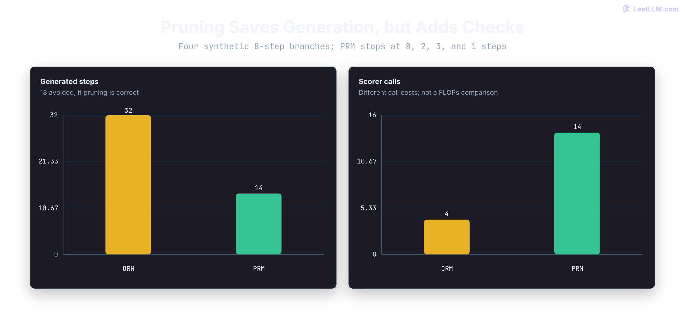
The next cell counts generated steps when three of four branches are pruned early. It doesn't measure FLOPs: steps can have different lengths, and scoring has its own cost. This fixture saves generation only if pruning is correct. A deployment eval must also count false pruning of branches that would have ended correct.

branch_lengths = [8, 8, 8, 8]
prune_at_step = [None, 2, 3, 1]

orm_generated_steps = sum(branch_lengths)
prm_generated_steps = sum(
    full_length if stop is None else stop
    for full_length, stop in zip(branch_lengths, prune_at_step, strict=True)
)
print(f"orm_steps={orm_generated_steps} prm_steps={prm_generated_steps}")
print(f"saved_steps={orm_generated_steps - prm_generated_steps}")
print(f"orm_score_calls={len(branch_lengths)} prm_score_calls={prm_generated_steps}")

orm_steps=32 prm_steps=14
saved_steps=18
orm_score_calls=4 prm_score_calls=14

DeepSeek-R1-Zero and DeepSeek-R1

DeepSeek's contribution separates into two experiments. DeepSeek-R1-Zero tested whether large-scale RL with verifiable rewards could induce strong reasoning without supervised cold start data.^{[4]Reference 4DeepSeek-R1: Incentivizing Reasoning Capability in LLMs via Reinforcement Learninghttps://arxiv.org/abs/2501.12948} DeepSeek-R1 kept the reasoning RL idea, then added data and post-training to make the behavior more stable and readable.^{[4]Reference 4DeepSeek-R1: Incentivizing Reasoning Capability in LLMs via Reinforcement Learninghttps://arxiv.org/abs/2501.12948}

Training pipeline

The final DeepSeek-R1 pipeline therefore isn't “pure RL” end to end. The paper describes two supervised fine-tuning (SFT) stages around two RL stages. Each stage answers a concrete product problem: seed readable traces, reinforce checkable reasoning, filter useful rollouts, then broaden behavior.

1. Base model: Start with DeepSeek-V3-Base, a 671B Mixture-of-Experts (MoE) model with 37B active parameters per token.^{[4]Reference 4DeepSeek-R1: Incentivizing Reasoning Capability in LLMs via Reinforcement Learninghttps://arxiv.org/abs/2501.12948}
2. Cold-start Supervised Fine-Tuning (SFT): Collect thousands of long CoT examples and fine-tune the base model. The seed traces address the readability and language-mixing issues reported for R1-Zero.
3. Reasoning-oriented RL: Run GRPO (Group Relative Policy Optimization)-based RL on reasoning tasks. R1 also adds a language-consistency reward to improve readability, alongside accuracy rewards; that is a trade-off rather than correctness supervision alone.^{[4]Reference 4DeepSeek-R1: Incentivizing Reasoning Capability in LLMs via Reinforcement Learninghttps://arxiv.org/abs/2501.12948}
4. Rejection sampling + second SFT: Use the RL checkpoint to generate high-quality reasoning traces, mix them with supervised data from DeepSeek-V3 for non-reasoning domains, and retrain the base model. This recovers broader language behavior around the specialized reasoning policy.
5. Final RL for all scenarios: Run another RL stage across a broader prompt mix. Reasoning retains rule-based rewards; general tasks use reward models for preferences. Helpfulness is assessed on the final summary, while harmlessness assessment covers the full response.^{[4]Reference 4DeepSeek-R1: Incentivizing Reasoning Capability in LLMs via Reinforcement Learninghttps://arxiv.org/abs/2501.12948}

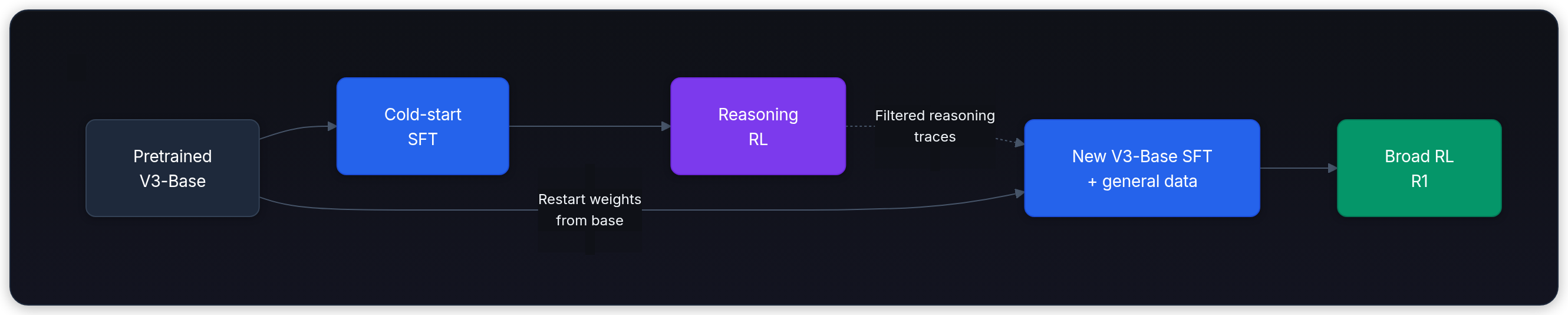
The dotted edge carries training examples; the second SFT starts again from V3-Base weights and adds general-domain data. “Pure RL” describes R1-Zero's reasoning post-training, not training from scratch: both models started from a pretrained base. R1 also used supervised stages around its RL stages.^{[4]Reference 4DeepSeek-R1: Incentivizing Reasoning Capability in LLMs via Reinforcement Learninghttps://arxiv.org/abs/2501.12948}

Emergent reasoning

R1-Zero displayed self-verification, backtracking, and longer rollouts, while the paper also reports readability issues and occasional language mixing.^{[4]Reference 4DeepSeek-R1: Incentivizing Reasoning Capability in LLMs via Reinforcement Learninghttps://arxiv.org/abs/2501.12948} Both observations belong in the same diagnosis: verifiable rewards can induce useful reasoning, but raw RL rollouts still need cleanup before they serve as a general-purpose product.

Compute-optimal inference: when to think harder

More thinking changes different workloads in different ways. Ghosal et al. studied three R1-distilled models on GSM8K, MATH-500, and AIME 2024, including forcing longer traces by suppressing the end-of-thinking delimiter and inserting Wait. Their results include initial accuracy gains followed by decline; their analysis attributes part of the early gain to higher output variance and recommends parallel sampling over forced extension.^{[5]Reference 5Does Thinking More Always Help? Mirage of Test-Time Scaling in Reasoning Modelshttps://arxiv.org/abs/2506.04210} This experiment doesn't establish that raising a current provider's supported effort setting always follows that same curve.

An Anthropic Fellows study constructed tasks where longer reasoning amplified distractions and errors, including distractor-heavy counting and constraint-tracking tasks.^{[13]Reference 13Inverse Scaling in Test-Time Computehttps://alignment.anthropic.com/2025/inverse-scaling/} Budget is therefore an evaluated operating point, not a slider to max out.

Use task shape to choose a starting experiment, then check quality and latency on your workload:

The cross-over point

A task family may have a measured compute budget where a smaller model plus a test-time policy beats a larger single-pass model:

Here, $Q$ is measured quality and $C^*$ is one evaluated inference budget. A crossover at $C^*$ isn't a promise that every larger budget keeps helping. Quality can plateau or fall, and the preferred path changes with task difficulty, latency limits, verifier quality, and request volume.

Snell et al. compared PaLM 2-S* policies on MATH against a model roughly 14× larger answering once. Their FLOPs exchange matches pretraining plus expected inference, so the available smaller-model budget depends on the lifetime inference-to-training token ratio. It isn't simply equal per-request latency or equal serving cost. Their difficulty analysis also excludes the cost of estimating difficulty.^{[2]Reference 2Scaling LLM Test-Time Compute Optimally Can Be More Effective Than Scaling Model Parameters.https://arxiv.org/abs/2408.03314} A deployed router must charge for that estimation, verifier calls, and queue effects before claiming the policy is cheaper.

The router turns measurements into a product decision. The next cell uses invented policy rows to test a minimum-cost choice. In production, quality belongs to an evaluated task slice, not a prediction guaranteed for an individual request. If no validated route meets the constraints, return an explicit fallback instead of silently selecting an ineligible path.

routes = [
    {"name": "single-pass", "quality": 0.78, "latency_ms": 240, "cost": 0.002},
    {"name": "bounded-reasoning", "quality": 0.86, "latency_ms": 780, "cost": 0.010},
    {"name": "guided-search", "quality": 0.90, "latency_ms": 2600, "cost": 0.045},
]
latency_slo_ms = 1000
minimum_quality = 0.84

eligible = [
    route for route in routes
    if route["latency_ms"] <= latency_slo_ms and route["quality"] >= minimum_quality
]
if not eligible:
    raise ValueError("no validated route: defer or request human review")
chosen = min(eligible, key=lambda route: route["cost"])
print(f"route={chosen['name']} quality={chosen['quality']:.0%}")
print(f"latency_ms={chosen['latency_ms']} cost=${chosen['cost']:.3f}")

route=bounded-reasoning quality=86%
latency_ms=780 cost=$0.010

That route avoids an intelligence tax: extra latency and cost for a reasoning path when a single-pass baseline already matches measured quality. Simple classification and extraction are useful places to test a cheap baseline, rather than assume every task with that label is easy. capacity_math earns the expensive path only if its measured gain survives the SLO.

Production considerations

Once a request takes the expensive route, its extra work becomes a serving problem. Longer traces and more branches can raise cache residency, visible-output delay, and cost even when the final answer stays short. A quality gain that exhausts the queue is not a free gain.

KV cache pressure and prefix sharing

Reasoning workloads stress an inference engine differently from ordinary chat because they can generate many intermediate tokens before or between visible outputs. Start with the cache, not the final answer length.

For a conventional full-attention transformer with uniform layer geometry, each cached token has a Key vector and a Value vector per KV head and layer:

Here $L$ is the number of layers, $n_{kv}$ the number of KV heads, $d_h$ the head dimension, and $b$ bytes per value. This cache grows linearly with retained sequence length. Sliding windows, compressed caches, heterogeneous layers, and state-space architectures need different accounting. With L=32, eight KV heads, head dimension 128, and two-byte values, the formula gives 128 KiB per token. This excludes allocator and metadata overhead.

PagedAttention stores KV cache in fixed-size blocks to reduce fragmentation and support sharing.^{[14]Reference 14Efficient Memory Management for Large Language Model Serving with PagedAttention.https://arxiv.org/abs/2309.06180} SGLang's RadixAttention also reuses matching prefixes.^{[15]Reference 15SGLang: Efficient Execution of Structured Language Model Programshttps://arxiv.org/abs/2312.07104} Best-of-N can share the prompt even when candidates diverge immediately afterward. The next cell calculates ideal storage for capacity_math; it doesn't measure an allocator. Partial blocks, copy-on-write, eviction, and concurrent scheduling can change realized savings.

prompt_tokens = 4000
continuation_tokens = 1000
branches = 8
kv_bytes_per_token = 2 * 32 * 8 * 128 * 2

without_sharing = branches * (prompt_tokens + continuation_tokens)
with_sharing = prompt_tokens + branches * continuation_tokens
saved_gib = (without_sharing - with_sharing) * kv_bytes_per_token / 1024 ** 3
print(f"tokens_without_sharing={without_sharing:,}")
print(f"tokens_with_sharing={with_sharing:,} saved_kv_gib={saved_gib:.2f}")

tokens_without_sharing=40,000
tokens_with_sharing=12,000 saved_kv_gib=3.42

TTFT vs. inter-token latency

Test-time compute changes which latency the user feels first. A provider or wrapper that generates non-visible reasoning before revealing an answer can push TTFT (time to first token) up substantially.^{[6]Reference 6Reasoning modelshttps://developers.openai.com/api/docs/guides/reasoning} An interleaved mode can pause between visible chunks or tool calls. ITL (inter-token latency) may still look healthy once answer text streams, while the request already feels slow.

For engines that generate reasoning autoregressively, that work is decode load. Under contention it can raise other tenants' ITL and reduce goodput: completed requests per second that satisfy the chosen latency and quality constraints. Goodput is not the offered arrival rate. A reasoning router must leave headroom for co-tenant latency as well as its own TTFT budget.

The next cell assumes the entire token cap is consumed before any visible token, at a constant 80 tokens per second, plus 180 ms of other delay. It compares that scenario with a 3000 ms TTFT limit. A cap is not actual usage, and throughput changes under load, so this is neither a latency prediction nor an SLO guarantee.

base_ttft_ms = 180
decode_tokens_per_second = 80
budgets = [0, 128, 512, 1024]
ttft_slo_ms = 3000

for budget in budgets:
    ttft_ms = base_ttft_ms + budget / decode_tokens_per_second * 1000
    status = "fits" if ttft_ms <= ttft_slo_ms else "reject"
    print(f"budget={budget:>4} ttft_ms={ttft_ms:>7.0f} {status}")

budget=   0 ttft_ms=    180 fits
budget= 128 ttft_ms=   1780 fits
budget= 512 ttft_ms=   6580 reject
budget=1024 ttft_ms=  12980 reject

Latency vs. quality trade-off

Reasoning models add latency, but the exact numbers depend on hardware, batching policy, and provider implementation:

For strict interactive latency budgets, a long reasoning path needs measured gains to justify its delay. Larger budgets fit better in:

• Batch processing (code review, data analysis)
• High-stakes analyst workflows (incident review, safety analysis, compliance analysis)
• Asynchronous workflows (software engineering, research)

Cost implications

Extended reasoning can be expensive even when the final answer is short. Hosted APIs may charge directly for hidden reasoning tokens. OpenAI's reasoning docs, for example, count them as output tokens even though the API doesn't return them verbatim.^{[6]Reference 6Reasoning modelshttps://developers.openai.com/api/docs/guides/reasoning} Open-weight deployments pay through additional runtime work and, for full-attention paths, longer KV residency. Under constrained capacity, that can lower the same GPU's goodput; measure the change rather than infer a fixed concurrency penalty from final-answer length.

Three controls keep that bill tied to evidence:

1. Routing: spend extra compute on task slices with demonstrated benefit; high stakes may instead require human review
2. Token budgets: cap how long a rollout may think before the marginal gain stops being worth it
3. Early stopping: terminate search when verifier scores stop improving

Without them, an ambiguous or unsolvable prompt can burn inference budget without producing a better answer.

Distillation: making reasoning affordable

Distillation moves work from serving to training. A larger reasoner writes detailed capacity_math traces; a smaller student trains on them and can solve similar sizing problems with less live compute. The student may inherit a solution style without inheriting the teacher's full search behavior.

The January 2025 DeepSeek-R1 paper reported the following AIME 2024 results. These are historical paper results, not local reruns or current model rankings. Its pass@1 estimates average correctness across sampled responses at temperature 0.6 and top-p 0.95, rather than reporting one greedy attempt.^{[4]Reference 4DeepSeek-R1: Incentivizing Reasoning Capability in LLMs via Reinforcement Learninghttps://arxiv.org/abs/2501.12948}

In DeepSeek's reported AIME evaluation, the 7B and 32B distilled models retain substantial benchmark accuracy at lower parameter counts than R1. Parameter count is only a proxy: deployment cost also depends on active parameters, quantization, batch size, and engine choice. Distillation can lower reasoning cost, but routing and token budgets still decide the serving bill.

Trace cloning has a scaling ceiling. Setlur et al. compare verifier-free methods that distill or clone successful traces with verifier-based methods using rewards, RL, or search.^{[16]Reference 16Scaling Test-Time Compute Without Verification or RL is Suboptimalhttps://arxiv.org/abs/2502.12118} Under their assumptions and evaluated reasoning tasks, verifier-free methods become increasingly suboptimal as rollout length and test-time budget grow: the student sees successful traces, but not which alternative traces a verifier would reward.

That result doesn't make distillation useless or establish a universal ceiling for every student. It motivates a comparison: filter traces with reliable checks, retain a verifier during evaluation, and compare against verifier-guided training when trustworthy rewards are available.

Before spending on eight branches

Return to capacity_math: the calculator checks 12,000 cached token positions under perfect sharing, and the stated architecture converts that to about 1.46 GiB. The popular 5,000-position answer fails the arithmetic. The high-scoring 40,000-position answer fails the stated sharing assumption. More candidates help only when the return policy retains the useful evidence.

Before choosing the expensive route, answer three questions:

• What can check the result? A calculator can check this declared geometry; actual capacity needs the engine's allocation and headroom. A process score may measure recoverability rather than step validity.
• What happens at the limit? Effort guides computation, while a hard output cutoff may leave no answer. Completion status and correctness need separate checks.
• Whose budget pays? Charge difficulty estimation, discarded candidates, scoring, and retries. Measure the request's latency and its effect on other queued requests, alongside selected correctness.

Passing these arithmetic fixtures doesn't validate their invented quality or latency values. All executable examples here are CPU-only arithmetic or scripted search, with no model calls, trained verifier, GPU benchmark, or production routing evidence.