Personalize this lesson
Adapt explanations and teaching visuals to your background and preferred voice.
The last chapter taught an access-policy assistant to answer with the same chat template at train and serve time. Now consider a failure before generation: the assistant receives the right question but retrieves the wrong policy clause. "My service-account key is 18 days old. Can I keep using it?" should land near "Keys older than 14 days require a rotation ticket," not near an auto-merge rule.
Each clause is stored as a long embedding. An engineer proposes shortening every vector to save memory. What evidence would make that safe? A cleaner-looking plot isn't enough; the rotation clause still has to survive the top- retrieval that supplies the answer.
Keep two jobs separate:
- Can we store and search shorter vectors while still returning the same useful policy chunks?
- Can we draw a two-dimensional map that helps an engineer inspect confusing clusters?
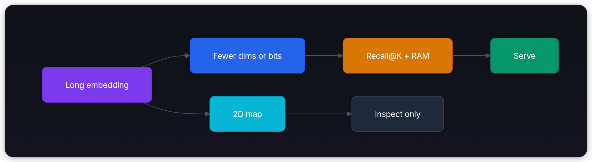
Both jobs use dimensionality reduction, but they don't share a success criterion. A production vector is approved by retrieval quality and cost. A plot is approved by what it lets you investigate, with important conclusions checked back in the original embedding space.
Start by measuring the policy index's storage and retrieval results. Every proposed representation will be compared with that baseline.
Start with the budget, not an algorithm
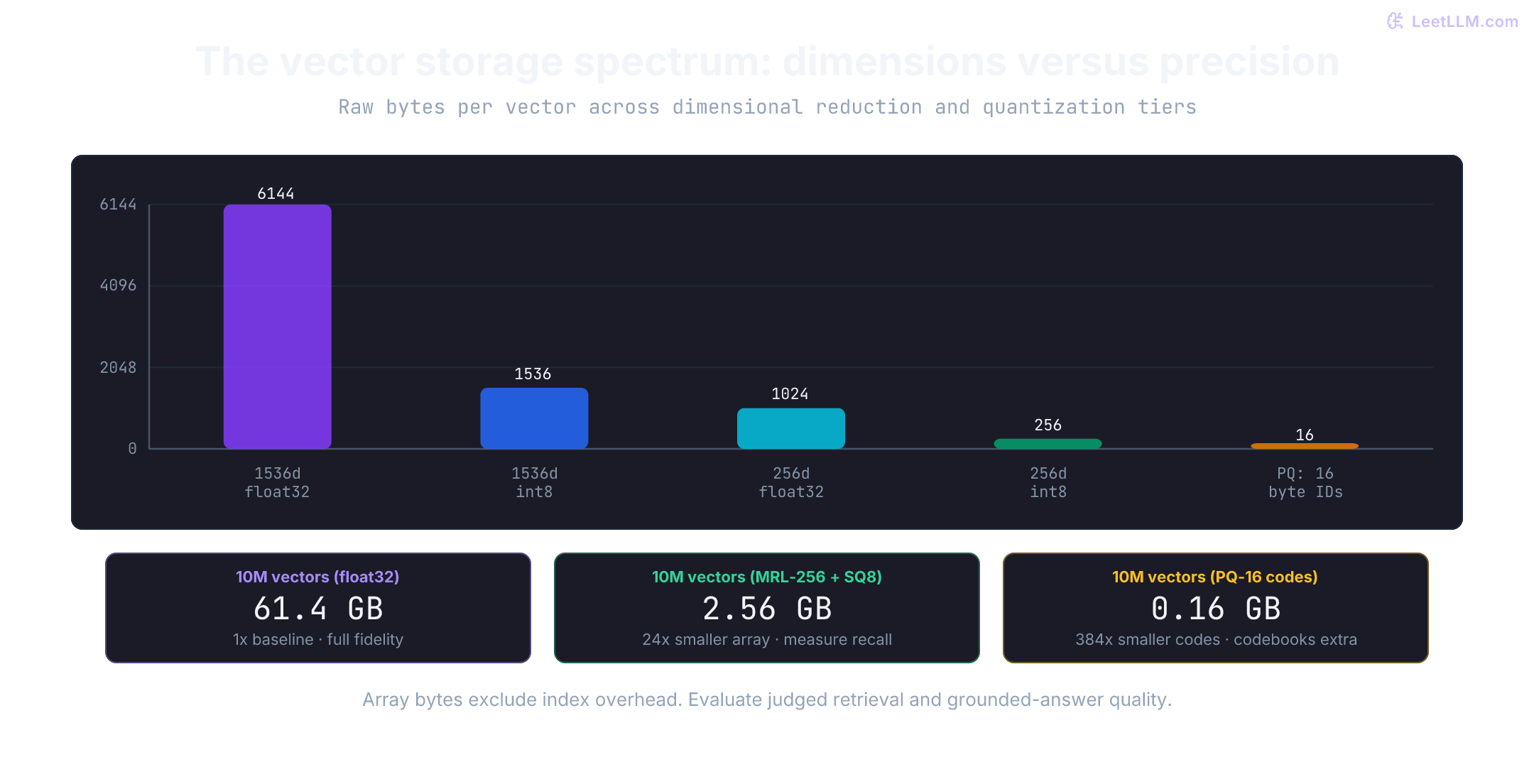
Before choosing a reducer, put the storage pressure on paper. An embedding is an array of numbers, and float32 storage costs four bytes per dimension. Storing ten million 1,536-dimensional policy or document vectors therefore costs:
That's 61.44 GB using decimal gigabytes, before the index graph, metadata, replicas, or backups.
Many coordinates also make each distance calculation expensive. Distance concentration can add difficulty, but it depends on the data distribution. For a concrete model, take independent vectors with and . Their squared separation has:
Under these assumptions, squared distances concentrate relative to their mean as increases, and distances cluster around . This isn't a theorem that every learned embedding loses its useful neighbors. An encoder can organize a large coordinate space around a much smaller intrinsic structure; check its actual distance distribution and retrieval results.
Graph-based approximate nearest neighbor (ANN) indexes such as Hierarchical Navigable Small World (HNSW) add another memory budget: neighbor IDs, levels, and bookkeeping. Higher graph degree and search effort can improve recall at a cost, but dimensionality alone doesn't prescribe their values. Faiss's index table includes graph storage separately from float32 bytes.[1] That overhead can dominate aggressively compressed codes; it doesn't automatically double a 6,144-byte full vector.
Engineers have two complementary levers to escape this memory wall:
- Dimensionality reduction: Shrink the coordinate count (for example, from 1,536 down to 256 dimensions).
- Quantization: Shrink the bit-precision of each coordinate (for example, mapping 32-bit floats to 8-bit integers or 1-byte codes).
Cutting the vector from 1,536 to 256 dimensions makes the raw array six times smaller. Run the arithmetic first. It turns "embeddings feel large" into a concrete engineering constraint.
def decimal_gb(byte_count: int) -> float:
    return byte_count / 1_000_000_000

documents = 10_000_000
bytes_per_float32 = 4
full_dim = 1_536
candidate_dim = 256

full_bytes = documents * full_dim * bytes_per_float32
candidate_bytes = documents * candidate_dim * bytes_per_float32

print(f"Full float32 array: {decimal_gb(full_bytes):.2f} GB")
print(f"256-d float32 array: {decimal_gb(candidate_bytes):.2f} GB")
print(f"Raw-vector reduction: {full_bytes / candidate_bytes:.1f}x")Full float32 array: 61.44 GB
256-d float32 array: 10.24 GB
Raw-vector reduction: 6.0xThe first applied habit is simple: separate a cost metric from a quality metric.
| Question | Useful metric |
|---|---|
| Will vectors fit in memory? | Bytes per vector, total RAM, index overhead |
| Will useful evidence still be retrieved? | Recall@K, nDCG@K, answer success on grounded evaluations |
| Will an engineer understand failures? | A labeled plot plus checks in the original space |
Why can't a six-times smaller vector index be approved from storage savings alone?
Answer
Storage reports the benefit, not the semantic loss. A shorter index can omit the policy chunk needed to answer a request correctly. Approval requires retrieval or downstream answer measurements on representative queries.
Build a retrieval baseline
Storage has a number now, but quality still needs a reference. Before compressing anything, define what "the same useful neighbors" means. The small fixture below represents six policy clauses. Its coordinates are hand-written so you can see the experiment without needing an API key: the first two coordinates concern key rotation, the next two concern merge gates, and the last two concern access escalations.
Cosine similarity compares directions rather than raw lengths. We L2-normalize each vector, score one 18-day-key query, and save the top results as the baseline that reduction must try to preserve.
Before running the cell, predict its first two clauses. The query points toward the first two coordinates, so the two rotation clauses should lead; the later merge and access clauses are controls for a false neighbor.
import math

documents = [
    "Keys older than 14 days require a rotation ticket before continued use.",
    "Rotate a stale service-account key and open a ticket before reuse.",
    "Auto-merge only when tests, security scan, and reviewer approval all pass.",
    "A failed security scan blocks merge even if tests are green.",
    "Access escalations need an owner and an expiry; never grant standing admin.",
    "Standing production admin is forbidden; use a time-bounded escalation.",
]

vectors = [
    [1.00, 0.92, 0.04, 0.00, 0.02, 0.00],
    [0.92, 0.80, 0.04, 0.01, 0.02, 0.00],
    [0.02, 0.00, 1.00, 0.88, 0.04, 0.00],
    [0.02, 0.02, 0.91, 0.98, 0.00, 0.00],
    [0.00, 0.00, 0.04, 0.02, 1.00, 0.89],
    [0.02, 0.00, 0.00, 0.02, 0.91, 1.00],
]
query = [0.98, 1.00, 0.03, 0.00, 0.01, 0.00]

def dot(left: list[float], right: list[float]) -> float:
    return sum(a * b for a, b in zip(left, right))

def normalize(vector: list[float]) -> list[float]:
    scale = math.sqrt(dot(vector, vector))
    return [value / scale for value in vector]

query_hat = normalize(query)
scores = [dot(normalize(vector), query_hat) for vector in vectors]
ranking = sorted(range(len(scores)), key=lambda index: -scores[index])

for rank, index in enumerate(ranking[:3], start=1):
print(f"{rank}. {documents[index]} score={scores[index]:.3f}")1. Keys older than 14 days require a rotation ticket before continued use. score=0.999
2. Rotate a stale service-account key and open a ticket before reuse. score=0.997
3. A failed security scan blocks merge even if tests are green. score=0.036In a real evaluation set, each query has judged relevant documents. For a query with two relevant rotation clauses, recall@2 = 1.0 means both appear in the top two returned results. That's the comparison target for every compressed representation here.
PCA: learn a shorter linear coordinate system
Suppose two coordinates for three clauses are [1, 1], [2, 2], and [3, 3]. Their mean is [2, 2]. Subtract it to get [-1, -1], [0, 0], and [1, 1]. All variation lies along the diagonal: the two original coordinates repeat the same information. Projecting onto the unit direction [1/√2, 1/√2] gives [-√2, 0, √2]. One coordinate preserves all the variation in this small example.
Principal component analysis (PCA) discovers these variance-maximizing directions from data. Let be the document embedding matrix. We center it by subtracting the column mean , giving the centered matrix . The sample covariance matrix is:
Rather than explicitly constructing this covariance matrix in memory, Singular Value Decomposition (SVD) factors directly:[2]
Use a thin SVD with : , , and . The columns of and are orthonormal; contains non-negative singular values in descending order. Centering limits the number of nonzero values to at most . Substitution gives:
The supplied columns of are covariance eigenvectors with ; any remaining directions have zero eigenvalues. Direct SVD avoids forming , which squares the singular-value condition number. This is a solver choice: some library PCA solvers do form covariance matrices.[3] Projecting onto the top nonzero right singular vectors gives:
Sample variance uses the denominator; a population mean-square convention uses . That common factor cancels in the explained-variance ratio (EVR), which measures the fraction of corpus spread retained:
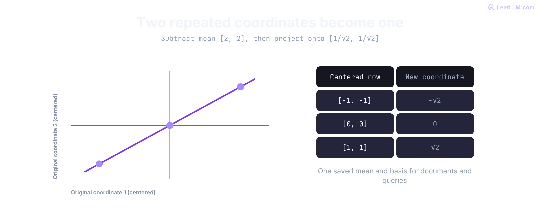
One fitted mean and basis must transform both sides of the search. Fitting PCA separately on document vectors and live queries creates different axes, so their dot products no longer compare like with like. Persist the transform fitted on representative documents and reuse it for indexed documents and future queries.
Fit on documents available at index-build time, choose the dimension using development queries, and reserve separate queries for the final evaluation. If PCA feeds a supervised model, fit it inside each training fold. PCA centers but doesn't automatically standardize coordinates; scaling or whitening is another change to evaluate.[3]
Centering changes cosine similarity even if every principal component is retained: cosine depends on the origin. After projection, normalize again for dot-product cosine search, and reject zero-length projected vectors rather than divide by zero.
Keep two common traps in mind before relying on PCA for production search:
- Uneven directional spread (anisotropy): Some embedding spaces have a strong mean or concentrate variation in a few directions. Measure the mean and singular-value spectrum for your encoder and corpus. Leading components might reflect length or other nuisance features, but they can also carry useful distinctions. A large component isn't automatically an artifact to remove.
- Variance doesn't equal relevance: PCA preserves directions with the highest corpus-wide spread. In policy retrieval, a high-variance direction might reflect whether a text discusses cloud infrastructure or HR benefits, while the critical distinction between "14-day key allowed" and "rotation ticket required" might lie along a low-variance direction. Discarding low-variance coordinates can silently discard the exact signal needed for retrieval.
The next cell adds small variations around the three policy themes, fits a two-dimensional PCA model, and retrieves with a query transformed by that same model. Predict the final label first: the query still describes rotation, even though its coordinates will change.
import numpy as np
import random

centers = [
    [1.0, 0.9, 0.0, 0.0, 0.0, 0.0],  # rotation
    [0.0, 0.0, 1.0, 0.9, 0.0, 0.0],  # merge
    [0.0, 0.0, 0.0, 0.0, 1.0, 0.9],  # access
]
labels = ["rotation"] * 20 + ["merge"] * 20 + ["access"] * 20
rng = random.Random(4)
documents = np.array([
    [center[j] + rng.gauss(0, 0.05) for j in range(6)]
    for center in centers
    for _ in range(20)
])
query = np.array([[0.96, 0.91, 0.02, 0.01, 0.00, 0.00]])

def normalize_rows(rows):
    rows = np.asarray(rows, dtype=float)
    if rows.ndim != 2 or rows.shape[1] == 0 or not np.isfinite(rows).all():
        raise ValueError("expected a finite matrix with nonempty vectors")
    # Scale first so squaring very large finite coordinates doesn't overflow.
    peaks = np.max(np.abs(rows), axis=1, keepdims=True)
    if (peaks == 0).any():
        raise ValueError("cosine requires nonzero vectors")
    rows = rows / peaks
    norms = np.linalg.norm(rows, axis=1, keepdims=True)
    return rows / norms

def fit_pca(rows, k):
    rows = np.asarray(rows, dtype=float)
    if rows.ndim != 2 or not np.isfinite(rows).all():
        raise ValueError("expected a finite document matrix")
    if type(k) is not int or not 1 <= k <= min(rows.shape[0] - 1, rows.shape[1]):
        raise ValueError("k exceeds the centered matrix's possible rank")
    mean = rows.mean(axis=0)
    _, singular_values, vt = np.linalg.svd(rows - mean, full_matrices=False)
    if singular_values[k - 1] <= 1e-12:
        raise ValueError("requested a zero-variance component")
    basis = vt[:k].T
    kept = (singular_values[:k] ** 2).sum() / (singular_values ** 2).sum()
    return mean, basis, kept

mean, basis, kept = fit_pca(documents, k=2)
reduced_documents = normalize_rows((documents - mean) @ basis)
reduced_query = normalize_rows((query - mean) @ basis)
best_index = int(np.argmax(reduced_documents @ reduced_query[0]))

print(f"Shape: {documents.shape} -> {reduced_documents.shape}")
print(f"Explained variance kept: {kept:.3f}")
print(f"Closest policy theme: {labels[best_index]}")Shape: (60, 6) -> (60, 2)
Explained variance kept: 0.992
Closest policy theme: rotationPCA optimizes variance, not relevance. A direction that rarely changes in the corpus can still distinguish "auto-merge allowed" from "security scan failed." Explained variance helps diagnose what the projection retained; retrieval recall decides whether the index is safe to ship.
Sweep dimensions against neighbor recall
One successful query doesn't establish a dimension. On a small data set, you can provide the relevance judgments yourself. This lab creates twenty policy intents in a noisy 24-dimensional space, gives each query three acceptable chunks, and tries PCA dimensions 2, 4, 8, and 12. Predict the tradeoff: the first cuts should save more coordinates, but may lose neighbors.
rng = random.Random(21)
dimensions = 24
intent_count = 20
acceptable_chunks = 3

def top_k(query_rows, doc_rows, k):
    scores = normalize_rows(query_rows) @ normalize_rows(doc_rows).T
    return np.argsort(-scores, axis=1, kind="stable")[:, :k]

intent_vectors = np.array([[rng.gauss(0, 1) for _ in range(dimensions)] for _ in range(intent_count)])
intent_vectors = normalize_rows(intent_vectors - intent_vectors.mean(axis=0))

documents: list[list[float]] = []
queries: list[list[float]] = []
relevant: list[set[int]] = []
for intent in intent_vectors:
    first_chunk = len(documents)
    for _ in range(acceptable_chunks):
        documents.append([intent[j] + rng.gauss(0, 0.11) for j in range(dimensions)])
    queries.append([intent[j] + rng.gauss(0, 0.03) for j in range(dimensions)])
    relevant.append(set(range(first_chunk, first_chunk + acceptable_chunks)))

documents, queries = np.array(documents), np.array(queries)

def mean_recall(returned):
    return np.mean([
        len(expected & set(found)) / len(expected)
        for expected, found in zip(relevant, returned)
    ])

print(f"Full-space recall@3: {mean_recall(top_k(queries, documents, 3)):.3f}")
for target_dim in [2, 4, 8, 12]:
    mean, basis, kept = fit_pca(documents, k=target_dim)
    short_docs = (documents - mean) @ basis
    short_queries = (queries - mean) @ basis
    returned = top_k(short_queries, short_docs, k=3)
    recall = mean_recall(returned)
    print(
        f"{target_dim:>2} dims: recall@3={recall:.3f}, "
        f"variance={kept:.3f}"
)Full-space recall@3: 1.000
2 dims: recall@3=0.383, variance=0.294
4 dims: recall@3=0.867, variance=0.495
8 dims: recall@3=1.000, variance=0.727
12 dims: recall@3=1.000, variance=0.871The generated fixture assigns relevance by intent: all three chunks belonging to a query's intent count as relevant. Variance measures retained squared spread about the document mean, while recall measures how many relevant chunks survive. Neither metric is the other one's denominator. These numbers aren't a benchmark for any embedding model.
Try k=6 using the same helpers before looking at higher dimensions. Then change the document-noise standard deviation from 0.11 to 0.20 and rerun the whole sweep. Check whether the dimension that first reaches your chosen recall floor changes. Use these queries for development; create fresh held-out queries before reporting a final result. More retained variance never decreases as k grows, but retrieval recall need not improve monotonically.
For a check on your changes: six dimensions give recall 0.967 at noise 0.11, but only 0.783 at noise 0.20. In the noisier fixture, even the full-space baseline falls to 0.967. Compression can't be blamed for every retrieval error.
A PCA model keeps 95 percent of explained variance but loses a rotation-ticket chunk that the release criteria require in the top five. Should it ship?
Answer
No. PCA preserved high-variance directions, but the product needs correct retrieval. Reduce less aggressively, try another method, or revise the index only after the retrieval metric meets the required threshold.
A two-dimensional map is an investigation tool
The baseline and PCA experiment protect serving quality with judged neighbors. Debugging needs a different view. A two-dimensional projection can help an engineer ask:
- Are 18-day-key queries scattered into the merge-gate cluster?
- Are clauses from a new policy version isolated from older versions?
- Which points should an engineer inspect in the original data?
It doesn't become a search index just because the plot looks separated. Compressing a high-dimensional semantic vector to two coordinates forces distortion, so use the map to choose cases for inspection and return to the original vectors for a decision.
Check the neighbors behind a picture
PCA supplies a linear map. Other methods, including t-distributed stochastic neighbor embedding (t-SNE) and Uniform Manifold Approximation and Projection (UMAP), use nonlinear neighborhood objectives. Before comparing algorithms, check whether a map preserves a relationship you can verify: each clause's nearest neighbor.
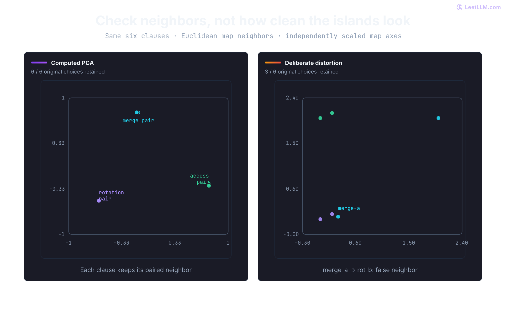
The lab uses the baseline's six policy vectors. Normalize them first so original-space Euclidean nearest neighbors agree with cosine nearest neighbors: for unit vectors, squared distance is 2 - 2 × cosine. Map-space neighbors use Euclidean distance without renormalizing the map. Predict which original pair the deliberate distortion breaks.
names = ["rot-a", "rot-b", "merge-a", "merge-b", "access-a", "access-b"]
vectors = [
    [1.00, 0.92, 0.04, 0.00, 0.02, 0.00],
    [0.92, 0.80, 0.04, 0.01, 0.02, 0.00],
    [0.02, 0.00, 1.00, 0.88, 0.04, 0.00],
    [0.02, 0.02, 0.91, 0.98, 0.00, 0.00],
    [0.00, 0.00, 0.04, 0.02, 1.00, 0.89],
    [0.02, 0.00, 0.00, 0.02, 0.91, 1.00],
]
pretty_map = [
    [0.00, 0.00],
    [0.20, 0.10],
    [0.30, 0.05],  # merge-a pulled into the rotation island
    [2.00, 2.00],
    [0.00, 2.00],
    [0.20, 2.10],
]

def nearest_names(rows: list[list[float]]) -> list[str]:
    neighbors: list[str] = []
    for i, left in enumerate(rows):
        best_j, best_d = -1, float("inf")
        for j, right in enumerate(rows):
            if i == j:
                continue
            dist = sum((a - b) ** 2 for a, b in zip(left, right))
            if dist < best_d:
                best_j, best_d = j, dist
        neighbors.append(names[best_j])
    return neighbors

def overlap(left: list[str], right: list[str]) -> float:
    return sum(a == b for a, b in zip(left, right)) / len(left)

unit_vectors = normalize_rows(vectors)
original = nearest_names(unit_vectors)
mean, basis, _ = fit_pca(unit_vectors, k=2)
pca_map = (unit_vectors - mean) @ basis
pca_neighbors = nearest_names(pca_map)
pretty_neighbors = nearest_names(pretty_map)

print("Original 1-NN:", list(zip(names, original)))
print(f"PCA 1-NN overlap:           {overlap(original, pca_neighbors):.2f}")
print(f"Pretty-island 1-NN overlap: {overlap(original, pretty_neighbors):.2f}")
print(f"Pretty-island neighbor of merge-a: {pretty_neighbors[2]}")Original 1-NN: [('rot-a', 'rot-b'), ('rot-b', 'rot-a'), ('merge-a', 'merge-b'), ('merge-b', 'merge-a'), ('access-a', 'access-b'), ('access-b', 'access-a')]
PCA 1-NN overlap: 1.00
Pretty-island 1-NN overlap: 0.50
Pretty-island neighbor of merge-a: rot-bPCA kept all six nearest-neighbor choices on this fixture. The hand-distorted map kept only three. This is neighbor overlap, not judged relevance recall: it measures agreement with the original geometry, whose neighbors might themselves be wrong for the task. Use it to check an inspection map, then evaluate queries against relevant documents before deploying a retrieval system.
t-SNE: match neighbor probabilities
Suppose a nearby pair gets probability 0.10 in the original space but only 0.01 in the map. Its contribution 0.10 × ln(0.10/0.01) ≈ 0.230 penalizes losing that relationship. Matching the pair at 0.10 makes its contribution zero. The total objective combines every pair; individual terms can be negative, but the full divergence is nonnegative.
t-distributed stochastic neighbor embedding (t-SNE) converts high-dimensional Euclidean distances into conditional probabilities using a Gaussian kernel. For , it chooses so matches the requested perplexity, then symmetrizes:[4]
Set self-pair probabilities to zero. The crowding problem arises when a map has too little room for the many moderately near points surrounding a record in a higher-dimensional neighborhood. It can't preserve all those distances while keeping the closest pairs close. In Gaussian SNE, the combined attractive forces from poorly placed moderate neighbors can crowd the map's center.[4]
van der Maaten and Hinton addressed this with a heavy-tailed Student-t distribution with one degree of freedom (a Cauchy kernel) in the map:
The slower-decaying map kernel lets moderate original-space similarities correspond to larger map distances. It doesn't make every original distance recoverable. The optimization minimizes the Kullback-Leibler (KL) divergence between and :
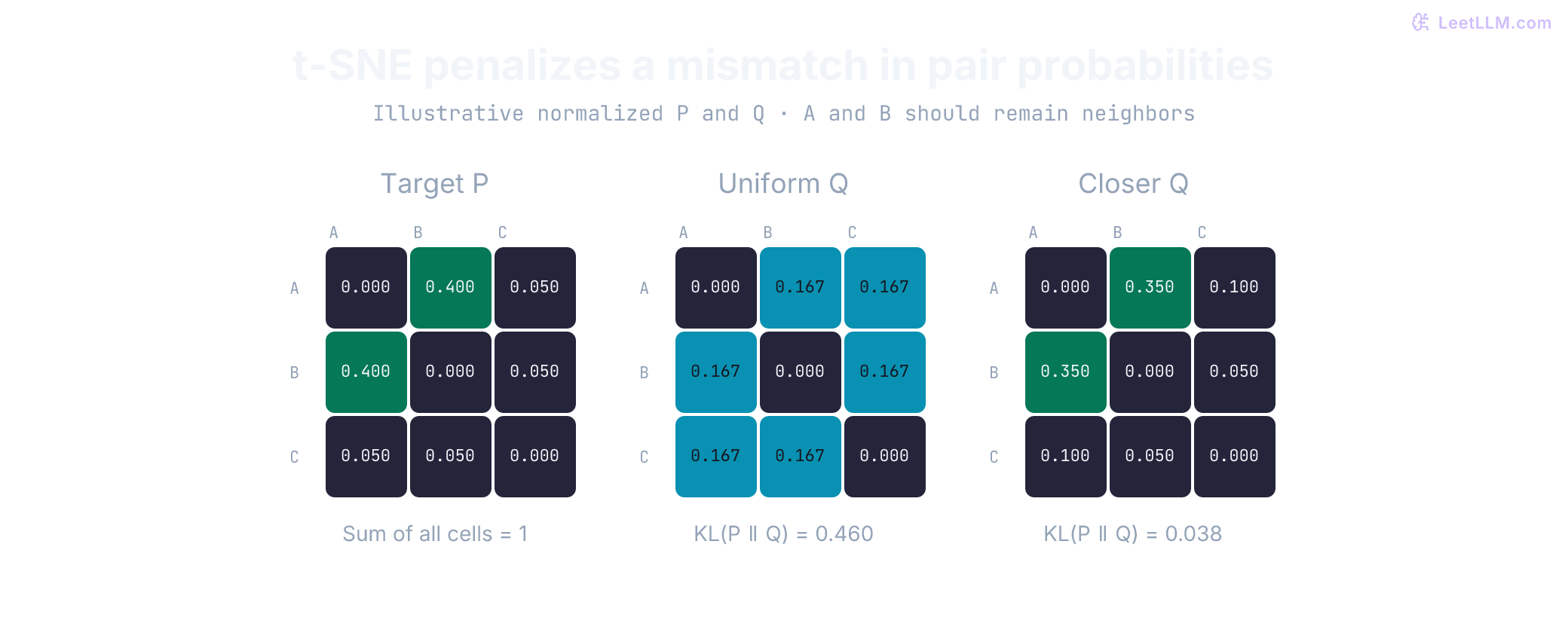
The perplexity parameter sets an effective neighborhood size, not a cluster count. Compare several perplexities and random seeds, and inspect known pairs. Neither island area nor empty space is a calibrated measure of density or semantic distance. The original nonparametric t-SNE formulation fits coordinates for the supplied records without an encoder for later queries. Use it for inspection here; out-of-sample extensions require a separate method.[4]
UMAP: optimize a weighted neighbor graph
While t-SNE focuses heavily on preserving local micro-neighborhoods, Uniform Manifold Approximation and Projection (UMAP) builds on Riemannian geometry and algebraic topology (fuzzy simplicial sets).[5]
The manifold assumptions motivate UMAP's construction; applying it doesn't establish that your embeddings satisfy them. With default local connectivity, reflects the nearest nonzero neighbor distance and calibrates the local neighborhood scale. For edges in the selected nearest-neighbor graph, directed membership strength is:
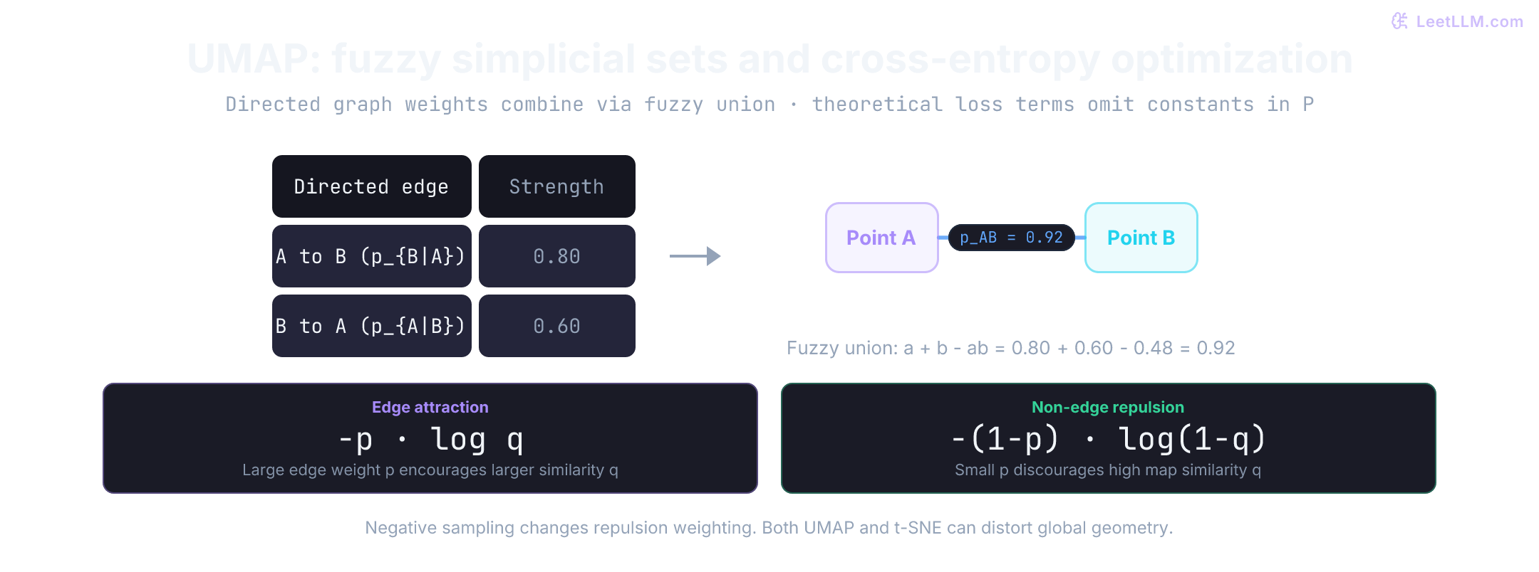
These directed strengths can differ. They are memberships in , rather than a distribution normalized across all pairs as in t-SNE. UMAP combines them using a fuzzy union (an algebraic t-conorm):
For example, directed strengths 0.80 and 0.60 combine into an undirected graph edge of weight .
Edges outside the selected directed neighborhood have zero membership. In low dimensions, UMAP uses . Its theoretical fuzzy-set cross-entropy objective, including constant terms in , is:
Use limiting values for zero-weight terms. Edge attraction encourages large for strong neighbors; non-edge repulsion discourages large for weak connections. The implementation samples negative edges instead of evaluating every pair, changing the effective repulsion weighting.[6] t-SNE also has repulsive forces through its normalized distribution.[4] Neither objective guarantees a faithful global layout.
n_neighbors controls the neighborhood size used to build the graph. Larger values consider broader relationships. min_dist controls how tightly points can pack in the low-dimensional representation; a small value can produce tighter-looking clusters without proving stronger semantic separation.[7] Standard UMAP can place later samples into a fitted map using its learned fuzzy complex, but that operation isn't a simple linear transform. Keep the source metric, preprocessing, parameters, and seed with the plot, and re-check important claims against original vectors.
| Goal | Appropriate first measurement | Suitable methods to test |
|---|---|---|
| Inspect clusters or outliers | Neighbor overlap plus human review | PCA, t-SNE, UMAP |
| Shorten vectors for retrieval | Recall@K or nDCG@K plus RAM and latency | Native shortening, PCA, random projection |
| Reduce memory further | Recall after compressed search and reranking | Scalar, PQ, binary quantization |
Random projection: a no-fit serving baseline
Suppose policy documents change frequently and fitting a corpus-dependent transform like PCA creates painful re-indexing operational overhead. While PCA requires data-driven calibration, a random projection samples a fixed matrix once and applies it identically to every indexed document and live query:
Here is the original dimension and is the target dimension. The theoretical foundation is the Johnson-Lindenstrauss lemma.[8]
For a fixed set of points and , a conventional sufficient dimension bound is:[9]
This establishes the existence of a linear map with the following squared Euclidean distance bounds. It doesn't promise that an arbitrary random draw succeeds with probability :
A sufficient dimension scales as without depending on . This is a conservative bound, not the minimum dimension a particular dataset needs. Success probabilities for randomized constructions require their own constants and failure-probability assumptions. Include both documents and queries in the fixed set when applying an all-pairs claim; it doesn't cover every unseen future query.
Does this bound justify compressing ten million records from 1,536 coordinates with ? Calculate before choosing an index:
import math

def sufficient_jl_dimension(points: int, epsilon: float) -> int:
    if type(points) is not int or points < 2:
        raise ValueError("points must be an integer of at least two")
    if type(epsilon) not in (int, float) or not 0 < epsilon < 1:
        raise ValueError("epsilon must be strictly between zero and one")
    denominator = epsilon**2 / 2 - epsilon**3 / 3
    if denominator == 0:
        raise ValueError("epsilon is too small for this floating-point calculation")
    bound = 4 * math.log(points) / denominator
    if not math.isfinite(bound):
        raise ValueError("dimension bound exceeds this floating-point calculation")
    return math.ceil(bound)

target = sufficient_jl_dimension(10_000_000, 0.15)
print("Conservative sufficient dimension:", target)
print("Below the original 1536 dimensions:", target < 1536)
print(f"Allowed distance change: {100 * (math.sqrt(0.85) - 1):.1f}% "
f"to {100 * (math.sqrt(1.15) - 1):+.1f}%")Conservative sufficient dimension: 6368
Below the original 1536 dimensions: False
Allowed distance change: -7.8% to +7.2%The bound doesn't certify useful compression at this tolerance. An empirical 256-dimensional candidate might still work on judged queries, but that conclusion must come from the experiment. Notice the square root: 15% squared-distance distortion is about -7.8% to +7.2% distance distortion.
The projection matrix can be constructed in two common ways:
- Gaussian random projection: Sample entries .
- Sparse random projection (Achlioptas): Sample entries from with probabilities . About two-thirds are zero on average. Sparse kernels can exploit that structure, but the zero fraction doesn't imply a threefold speedup.[10]
Even a successful squared-distance bound needn't preserve ranks. Candidates at squared Euclidean distances 1.00 and 1.15 have overlapping admissible intervals when : and . The inequalities permit their order to swap. Renormalizing projected vectors for cosine search changes the geometry again, so evaluate that exact pipeline.
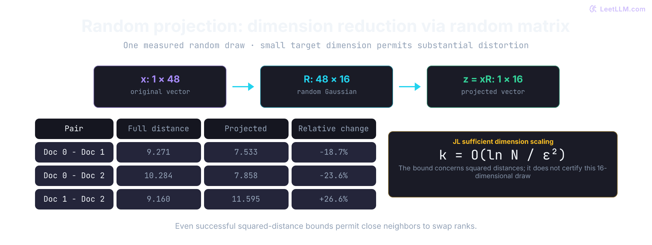
The experiment compares original cosine neighbors with a Gaussian random projection. A fixed seed makes the transform reproducible. The Gaussian entries are scaled by , matching the usual construction. Predict the result before running it: fewer bytes can come with a noticeable neighbor loss on this intentionally small target dimension.
import math
import random

rng = random.Random(33)
documents = [[rng.gauss(0, 1) for _ in range(48)] for _ in range(180)]
queries = [
    [documents[i][j] + rng.gauss(0, 0.03) for j in range(48)]
    for i in range(12)
]

def dot(left: list[float], right: list[float]) -> float:
    return sum(a * b for a, b in zip(left, right))

def normalize(vector: list[float]) -> list[float]:
    scale = math.sqrt(dot(vector, vector))
    return [value / scale for value in vector]

def neighbors(query_rows: list[list[float]], doc_rows: list[list[float]], k: int = 5) -> list[list[int]]:
    doc_hat = [normalize(row) for row in doc_rows]
    ranking: list[list[int]] = []
    for query in query_rows:
        query_hat = normalize(query)
        scores = [dot(doc, query_hat) for doc in doc_hat]
        order = sorted(range(len(scores)), key=lambda index: -scores[index])
        ranking.append(order[:k])
    return ranking

def apply_R(rows: list[list[float]], matrix: list[list[float]]) -> list[list[float]]:
    n_out = len(matrix[0])
    return [
        [sum(row[i] * matrix[i][j] for i in range(len(row))) for j in range(n_out)]
        for row in rows
    ]

gold = neighbors(queries, documents)
n_out = 16
proj_rng = random.Random(7)
scale = 1.0 / math.sqrt(n_out)
projection = [[proj_rng.gauss(0, scale) for _ in range(n_out)] for _ in range(48)]
short_docs = apply_R(documents, projection)
short_queries = apply_R(queries, projection)
predicted = neighbors(short_queries, short_docs)
recall = sum(
    len(set(left) & set(right)) / len(left)
    for left, right in zip(gold, predicted)
) / len(gold)

print(f"Bytes/vector: {48 * 4} -> {n_out * 4}")
print(f"Original-neighbor overlap@5: {recall:.3f}")Bytes/vector: 192 -> 64
Original-neighbor overlap@5: 0.317This cell measures overlap with the full-space top five, not semantic relevance: the random vectors have no judged policy labels. It isolates geometric loss from a 48-to-16 projection. For a deployment comparison, evaluate both random projection and PCA on the same labeled queries, and save the exact projection matrix rather than regenerate it independently in each service.
Compression after reduction: quantization
Projection changes how many coordinates a vector has. Quantization changes how precisely those coordinates are stored. You can use the two levers independently or together.
For example, a 256-dimensional float32 vector occupies bytes. Storing one signed byte per dimension cuts that to 256 bytes. Storing one bit per dimension cuts it to 32 bytes. The smaller representations buy memory by accepting more approximation.
Scalar and binary codes
Scalar quantization maps floating-point coordinates onto an integer grid. SQ8 denotes eight-bit scalar codes, with implementation-specific scaling and offsets. Our symmetric signed example uses , reserving the unused int8 value -128:
Eight-bit codes use one quarter of float32 array storage, before calibration metadata. Optimized integer kernels can lower bandwidth and scoring cost, but supported instructions, operand conventions, and throughput vary by CPU. Measure end-to-end latency and recall on the actual index; neither a universal twofold speedup nor a fixed recall penalty follows from the byte count.
Binary Quantization (BQ) pushes compression to the extreme by recording only a coordinate's sign:
Packing eight signs per byte makes a 256-dimensional code 32 bytes, versus 1,024 float32 bytes. Hamming distance between these codes can be computed with XOR and population count. It measures sign disagreement, not original cosine similarity: coordinate magnitudes are gone. The quality loss depends on the embedding distribution and search design.
In Qdrant, explicitly enable rescore: true when testing a compressed-search cascade. With oversampling: 2.4 and limit: 100, the documented example preselects 240 candidates and rescores them with original vectors. As of October 10, 2026, scalar and product quantization don't rescore by default; binary and the lower-bit TurboQuant options do.[11] Rescoring can fix order within the shortlist, but it can't retrieve an omitted document.
Current implementations also include rotation-based quantization. Qdrant 1.18 adds TurboQuant, which rotates vectors before low-bit coordinate coding and scores queries asymmetrically. Its 4-bit option halves coordinate-code storage relative to SQ8.[11][12] Rotation preserves Euclidean geometry before coding; quantization still introduces error. Compare supported metrics and measured retrieval quality rather than treating a newer quantizer as automatic approval.
The next lab stores four arrays as float32, quantizes them to int8, and packs their signs into bytes. They aren't unit vectors; the code is a storage demonstration, not a cosine-search benchmark. The symmetric scale is fitted on these documents and must be reused for queries. Out-of-range values would be clipped. Real indexes may use per-coordinate scales, offsets, or rotations instead.
import numpy as np

vectors = np.array([
    [0.90, 0.80, -0.10, -0.20, 0.04, 0.02, -0.05, 0.08],
    [0.85, 0.74, -0.04, -0.16, 0.01, 0.04, -0.02, 0.05],
    [-0.02, 0.04, 0.92, 0.81, -0.06, 0.01, 0.02, -0.04],
    [-0.05, 0.03, 0.88, 0.79, -0.03, 0.00, 0.06, -0.02],
], dtype=np.float32)

peak = np.abs(vectors).max()
if not np.isfinite(vectors).all() or peak <= 0:
    raise ValueError("calibration needs finite data with a positive maximum magnitude")
scale = 127 / peak
int8_vectors = np.clip(np.rint(vectors * scale), -127, 127).astype(np.int8)
binary_vectors = vectors > 0
packed = np.packbits(binary_vectors, axis=1)
query_bits = binary_vectors[0]
hamming = [
    sum(left != right for left, right in zip(row, query_bits))
    for row in binary_vectors
]

print(f"float32 bytes/vector: {vectors[0].nbytes}")
print(f"int8 bytes/vector:    {int8_vectors[0].nbytes}")
print(f"packed binary bytes/vector: {packed[0].nbytes}")
print(f"Binary Hamming distances from row 0: {[int(d) for d in hamming]}")float32 bytes/vector: 32
int8 bytes/vector: 8
packed binary bytes/vector: 1
Binary Hamming distances from row 0: [0, 0, 6, 7]Binary codes are tiny, but "same sign" is a much weaker statement than "same semantic evidence." For a policy assistant, retrieve more candidates with a compressed representation and rerank before final evidence selection if benchmarks justify that design. Measure the oversample factor against final recall and end-to-end latency; too small and true neighbors drop before rerank, too large and you pay second-stage cost without quality gain.
Product quantization: code sub-vectors
Binary codes illustrate the precision tradeoff on individual scalars. Product Quantization (PQ) splits a vector into disjoint coordinate blocks, learns centroids for each block using k-means, and replaces each block with its nearest centroid ID.[13] The coordinate subspaces are orthogonal; the blocks aren't independent semantic features.
In the standard configuration where , each centroid ID fits into exactly one byte (uint8). A 128-dimensional float32 vector split into subspaces (each of dimension 16) is therefore stored as an 8-byte code:
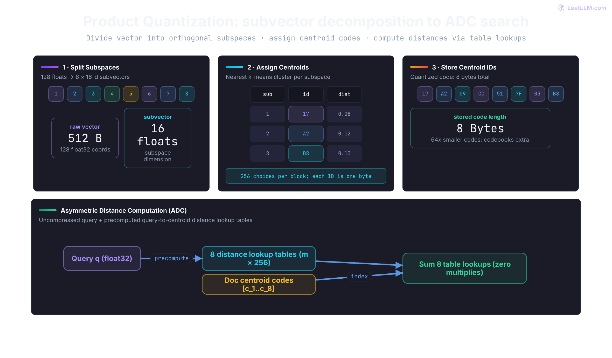
The original PQ paper introduces Asymmetric Distance Computation (ADC).[13] The query isn't PQ-encoded, while database vectors are. Our diagram uses a float32 query; that precision isn't a requirement of the definition. ADC avoids adding query-side centroid-assignment error.
When a query arrives:
- Partition into subvectors .
- For each subspace , precompute squared Euclidean distances between and all learned centroids into a small lookup table:
- For a document represented by centroid codes , its approximate distance to is simply the sum of table lookups:
At , a float32 table occupies bytes (96 KiB). Cache fit depends on the CPU and other active data. After building the tables, this simple scorer uses lookups and additions per candidate; table construction still requires distance calculations. Faiss documents further kernel and table-layout tradeoffs, so benchmark the complete search instead of assuming a latency.[14]
Symmetric Distance Computation (SDC) PQ-encodes both sides and can use precomputed centroid-to-centroid distances. It adds query-side approximation but changes query-time work. The original paper compares the methods; your quality and latency measurements decide the tradeoff, rather than a universal claim of twice the error.
Keep the metric consistent. The tables above approximate squared L2 distance. Original unit vectors have squared distance , but reconstructed centroid vectors needn't remain unit length. An L2 ADC ranking therefore isn't automatically a cosine ranking of reconstructed vectors. Use a scorer for the intended metric or rescore candidates with the original normalized vectors.
The lab uses two subspaces and four centroids per subspace. Each ID could fit in two bits, but the code deliberately stores one byte per ID for simple indexing.
import random
import numpy as np

rng = random.Random(12)
documents = (
    [[rng.gauss(1, 0.08), rng.gauss(1, 0.08), rng.gauss(0, 0.08), rng.gauss(0, 0.08)] for _ in range(20)]
    + [[rng.gauss(0, 0.08), rng.gauss(0, 0.08), rng.gauss(1, 0.08), rng.gauss(1, 0.08)] for _ in range(20)]
)
query = [0.94, 1.02, 0.01, -0.02]

def mean_col(rows: list[list[float]]) -> list[float]:
    n_rows, n_cols = len(rows), len(rows[0])
    return [sum(row[j] for row in rows) / n_rows for j in range(n_cols)]

def kmeans(rows: list[list[float]], k: int, seed: int) -> tuple[list[list[float]], list[int]]:
    local = random.Random(seed)
    centroids = [rows[local.randrange(len(rows))][:] ]
    while len(centroids) < k:
        weights = []
        for row in rows:
            nearest = min(
                sum((row[j] - center[j]) ** 2 for j in range(len(row)))
                for center in centroids
            )
            weights.append(nearest)
        pick = local.random() * (sum(weights) or 1.0)
        acc = 0.0
        chosen = rows[-1]
        for row, weight in zip(rows, weights):
            acc += weight
            if acc >= pick:
                chosen = row
                break
        centroids.append(chosen[:])
    labels = [0] * len(rows)
    for _ in range(15):
        for i, row in enumerate(rows):
            labels[i] = min(
                range(k),
                key=lambda c: sum((row[j] - centroids[c][j]) ** 2 for j in range(len(row))),
            )
        for cluster in range(k):
            members = [rows[i] for i, label in enumerate(labels) if label == cluster]
            if members:
                centroids[cluster] = mean_col(members)
    # Reassign against the final updated centroids.
    labels = [min(range(k), key=lambda c: sum(
        (value - center) ** 2 for value, center in zip(row, centroids[c])
    )) for row in rows]
    return centroids, labels

subspace_width = 2
codebooks: list[list[list[float]]] = []
codes: list[list[int]] = []
for start in range(0, len(documents[0]), subspace_width):
    block = [row[start:start + subspace_width] for row in documents]
    centroids, labels = kmeans(block, k=4, seed=start)
    codebooks.append(np.asarray(centroids, dtype=np.float32))
    codes.append(labels)

codes = np.asarray(codes, dtype=np.uint8).T.copy()
stored_vectors = np.asarray(documents, dtype=np.float32)

adc_scores = [0.0] * len(documents)
for subspace, start in enumerate(range(0, len(documents[0]), subspace_width)):
    query_block = query[start:start + subspace_width]
    table = [
        sum((center[j] - query_block[j]) ** 2 for j in range(subspace_width))
        for center in codebooks[subspace]
    ]
    for i, code in enumerate(codes[:, subspace]):
        adc_scores[i] += table[code]

best = min(range(len(adc_scores)), key=lambda i: adc_scores[i])
print(f"Document shape: ({len(documents)}, {len(documents[0])})")
print(f"Stored code shape: {codes.shape}")
print(f"Raw float32 bytes/vector: {stored_vectors[0].nbytes}")
print(f"Code bytes/vector: {codes[0].nbytes}")
print(f"Shared codebook bytes: {sum(book.nbytes for book in codebooks)}")
print(f"Nearest PQ-coded document group: {'rotation' if best < 20 else 'merge'}")Document shape: (40, 4)
Stored code shape: (40, 2)
Raw float32 bytes/vector: 16
Code bytes/vector: 2
Shared codebook bytes: 64
Nearest PQ-coded document group: rotationThe two code bytes replace sixteen float32 bytes per vector, but the shared codebooks add 64 bytes in this tiny fixture. Python objects and index metadata cost more; the printed nbytes values cover only numeric arrays. Fit codebooks on representative index-build data and reuse them for scoring, without fitting a new quantizer to live queries. An index may first shorten embeddings and then PQ-code them, provided the combined pipeline passes evaluation.
Why can a system use both PCA or native shortening and product quantization?
Answer
They reduce different costs. PCA or native shortening reduces the number of coordinates to compare. PQ stores those coordinates as compact centroid IDs, reducing memory further and enabling lookup-based approximate scoring.
Native shortening: train prefixes to be useful
PCA and random projection operate after encoding. Matryoshka Representation Learning (MRL) instead trains with losses at several prefix lengths, encouraging those shorter representations to remain useful.[15]
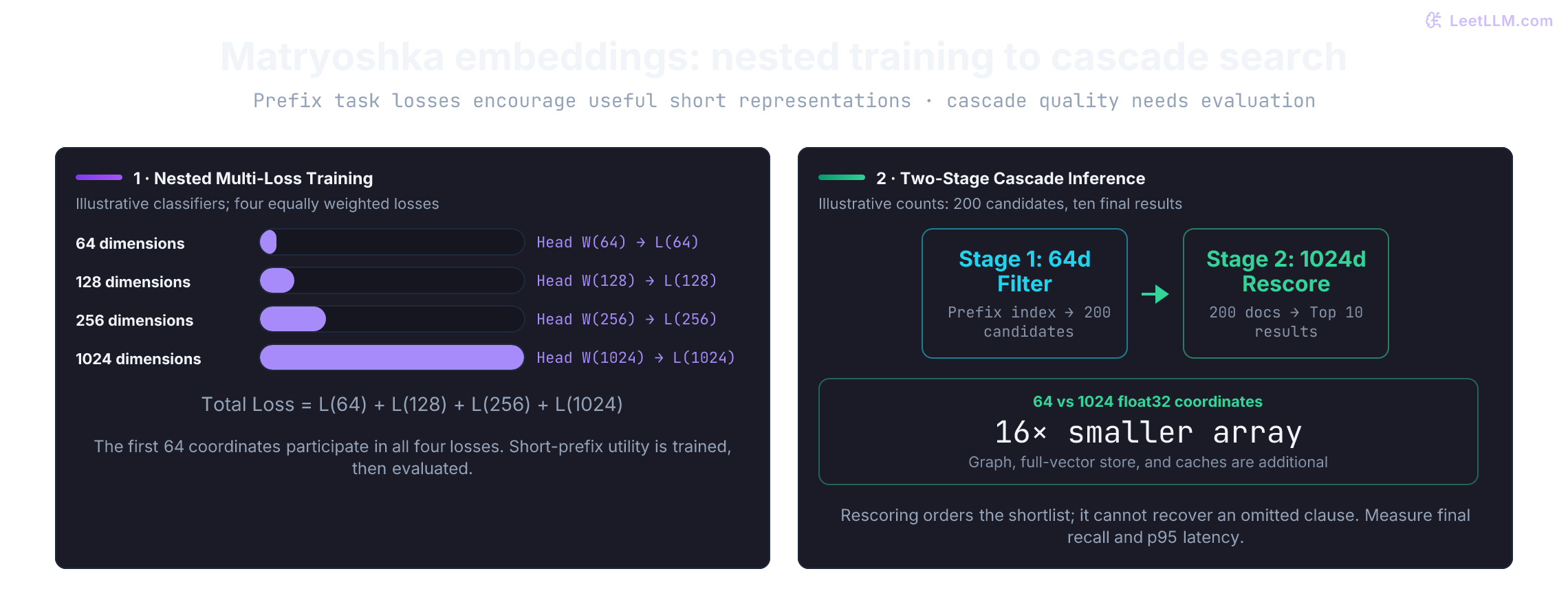
For an illustrative classification version, take , prefix lengths , non-negative weights , and classifier heads :
The first 64 coordinates participate in every loss term, creating pressure to support the task in short prefixes. This doesn't force a strict coarse-to-fine semantic ordering or guarantee nonzero gradients from every head. Separate classifiers are one formulation: the paper also describes shared-head MRL-E, and Sentence Transformers supports prefix losses for embedding training, including contrastive objectives.[15][16]
This training structure unlocks two-stage cascade search (also known as funnel retrieval) in production:
- Prefix candidate index: Index a supported 64- or 256-dimensional prefix, optionally quantized. Use the same prefix and normalization for queries. Search for a tunable shortlist, such as 200 candidates; this count is an experiment setting.
- Full-vector rescore: Fetch those candidates' original vectors from the retained store and compute the intended full-space similarity, selecting the final results.
A 64-dimensional float32 array is 16 times smaller than a 1,024-dimensional one (93.75% fewer array bytes). That isn't a total-RAM or recall result. Count the prefix index, graph, full-vector store, caches, and I/O. Measure final recall and latency; an accurate rescore can't recover a relevant clause excluded by the first stage.
The next cell is a negative control, not an MRL training demonstration. Rotation information starts in the first coordinates, merge information starts at coordinate three, and access information starts at coordinate five. Cutting every vector to two coordinates erases most access and merge signal. Predict why normalizing the short prefix can't restore that lost information.
import math
import random

rng = random.Random(15)
centers = [
    [1.0, 0.9, 0.3, 0.2, 0.0, 0.0, 0.0, 0.0],
    [0.0, 0.0, 1.0, 0.9, 0.3, 0.2, 0.0, 0.0],
    [0.0, 0.0, 0.0, 0.0, 1.0, 0.9, 0.3, 0.2],
]
documents = [
    [center[j] + rng.gauss(0, 0.04) for j in range(8)]
    for center in centers
    for _ in range(18)
]
queries = [
    [center[j] + rng.gauss(0, 0.02) for j in range(8)]
    for center in centers
    for _ in range(3)
]

def dot(left: list[float], right: list[float]) -> float:
    return sum(a * b for a, b in zip(left, right))

def normalize(vector: list[float]) -> list[float]:
    scale = math.sqrt(dot(vector, vector))
    return [value / scale for value in vector]

def top_k(rows: list[list[float]], corpus: list[list[float]], k: int = 3) -> list[list[int]]:
    corpus_hat = [normalize(row) for row in corpus]
    ranking: list[list[int]] = []
    for query in rows:
        query_hat = normalize(query)
        scores = [dot(doc, query_hat) for doc in corpus_hat]
        order = sorted(range(len(scores)), key=lambda index: -scores[index])
        ranking.append(order[:k])
    return ranking

gold = top_k(queries, documents)
for prefix in [2, 4, 8]:
    shortened = top_k(
        [query[:prefix] for query in queries],
        [doc[:prefix] for doc in documents],
    )
    recall = sum(
        len(set(expected) & set(found)) / 3
        for expected, found in zip(gold, shortened)
    ) / len(gold)
    print(f"Prefix {prefix}: original-neighbor overlap@3={recall:.3f}")

# Reuse the weakest prefix to generate candidates, then rescore in full space.
full_docs = [normalize(doc) for doc in documents]
full_queries = [normalize(query) for query in queries]
for candidate_count in [3, 12, len(documents)]:
    shortlists = top_k([q[:2] for q in queries], [d[:2] for d in documents], candidate_count)
    candidate_hits = sum(len(set(expected) & set(found))
                         for expected, found in zip(gold, shortlists))
    rescored = [sorted(found, key=lambda i: -dot(full_docs[i], q))[:3]
                for q, found in zip(full_queries, shortlists)]
    final_hits = sum(len(set(expected) & set(found))
                     for expected, found in zip(gold, rescored))
    assert final_hits == candidate_hits  # Exact scoring recovers every retained gold item.
    print(f"2d candidates={candidate_count:>2}: retained={candidate_hits}/27; "
          f"after full rescore={final_hits}/27")
Prefix 2: original-neighbor overlap@3=0.185
Prefix 4: original-neighbor overlap@3=0.407
Prefix 8: original-neighbor overlap@3=1.000
2d candidates= 3: retained=5/27; after full rescore=5/27
2d candidates=12: retained=17/27; after full rescore=17/27
2d candidates=54: retained=27/27; after full rescore=27/27
The second sweep uses the two-coordinate prefix only for candidate generation. Exact full-vector scoring recovers every original top-three neighbor that reaches the shortlist. It cannot recover a missing ID: the retained count is the ceiling for this exact rescore. The 54-candidate control searches the entire corpus, so it must reproduce the full-space result, while giving up the filtering benefit. Try a 24-candidate shortlist and measure that ceiling before claiming the cascade repaired the prefix. These synthetic neighbor counts still do not measure judged policy relevance.
One hosted API example is OpenAI's text-embedding-3 family. Its documentation, checked October 10, 2026, lists default lengths of 1,536 for text-embedding-3-small and 3,072 for text-embedding-3-large, with a dimensions parameter for shorter outputs.[17] The guide repeats a 2024 launch comparison: 256-dimensional text-embedding-3-large outperformed full-length text-embedding-ada-002 on MTEB. That historical result isn't a current leaderboard or a promise about rotation-ticket queries.
A request shape looks like this:
{
  "model": "text-embedding-3-large",
  "input": "My service-account key is 18 days old. Can I keep using it?",
  "dimensions": 256
}
⚠️ Common mistake: If you slice a returned vector yourself, L2-normalize the nonzero prefix again. OpenAI documents unit-normalized outputs even when using
dimensions; a manual cut doesn't preserve the original norm.[18]
The synthetic prefix numbers measure agreement with full-space neighbors, not semantic recall and not MRL performance. A documented shortening parameter or a prefix-trained model supplies a defensible candidate, not automatic approval for the 18-day-key query.
Choose a deployment experiment
The methods change different parts of the representation. Before choosing one, name the knob you need to turn: coordinates after encoding, coordinates learned into the encoder, or bits used to store each coordinate. The map methods stay on the investigation side.
A deployment experiment can combine them. Starting specifically from a 1,536-dimensional float32 baseline, try:
- Supported prefix: Use 256 coordinates from a prefix-trained model for documents and queries. This lowers subsequent storage and scoring work; it needn't lower encoder computation, because the encoder may still produce the full vector.
- Eight-bit coding: Quantize the prefix, reducing its array from 1,024 to 256 bytes per vector. The 24x reduction compares this code array with the original 6,144-byte array, excluding other storage.
- Candidate generation: Search the compressed prefix index for an illustrative 200 candidates. Tune search effort and shortlist length on development queries.
- Original-vector rescoring: Fetch retained 1,536-dimensional vectors from the same encoder checkpoint and rank candidates by full-space cosine similarity, selecting five policy chunks.
Persist the encoder version, prefix length, normalization, and quantizer parameters with the index. Benchmark the combined pipeline on held-out queries, including vector-fetch latency and grounded-answer quality. The architecture alone supplies no universal two-millisecond or 99%-recall guarantee.
These methods fall into three serving families and one diagnostic family:
| Tool family | What changes | Best first question |
|---|---|---|
| PCA or random projection | Number of served coordinates after encoding | How much recall survives at a lower dimension? |
| MRL-style native shortening | Number of coordinates emitted from a trained model | Does a supported prefix beat post-hoc alternatives at the same cost? |
| Scalar, binary, or product quantization | Precision or code used to store/search vectors | Can compressed candidate search plus reranking fit the RAM budget? |
| t-SNE or UMAP | Coordinates used for inspection maps | What failures should an engineer examine next? |
The table becomes useful when it turns into a decision someone else can audit. This lab accepts only configurations that meet both a recall floor and a raw-vector memory budget, then chooses the smallest accepted representation. Predict the winner from the two thresholds before reading the output.
import math

measurements = [
    {"method": "float32-full", "bytes_per_vector": 6144, "recall_at_10": 1.000},
    {"method": "native-256", "bytes_per_vector": 1024, "recall_at_10": 0.984},
    {"method": "pca-256", "bytes_per_vector": 1024, "recall_at_10": 0.971},
    {"method": "pq-16-code", "bytes_per_vector": 16, "recall_at_10": 0.939},
]

required_recall = 0.975
maximum_bytes = 1200

def passes_gate(row):
    recall = row.get("recall_at_10")
    byte_count = row.get("bytes_per_vector")
    valid_recall = type(recall) in (int, float) and 0 <= recall <= 1
    if not valid_recall or not math.isfinite(recall):
        return False
    valid_bytes = type(byte_count) is int and byte_count > 0
    return valid_bytes and recall >= required_recall and byte_count <= maximum_bytes

accepted = [row for row in measurements if passes_gate(row)]
choice = min(accepted, key=lambda row: row["bytes_per_vector"], default=None)

for row in measurements:
    status = "pass" if row in accepted else "reject"
    print(f"{row['method']:<14} recall={row['recall_at_10']:.3f} "
          f"bytes={row['bytes_per_vector']:<4} {status}")
print("Selected representation:", choice["method"] if choice else "none; keep the current index")float32-full recall=1.000 bytes=6144 reject
native-256 recall=0.984 bytes=1024 pass
pca-256 recall=0.971 bytes=1024 reject
pq-16-code recall=0.939 bytes=16 reject
Selected representation: native-256The values above are example measurements for the gate, not benchmark results for a real model. The gate rejects missing fields, invalid recall rates, and nonpositive or noninteger byte counts. Try setting the native candidate's recall to float("inf"), or its byte count to -1. Each must be rejected; the original threshold-only logic would have accepted them.
A serious report would include:
- A frozen set of realistic policy queries and judged clauses.
- Recall or nDCG at the candidate count sent to generation or reranking.
- Index RAM, build time, and query-latency percentiles for each candidate.
- A failure list: which queries lost relevant evidence, and what risk that creates.
- Re-evaluation when embedding models, policy documents, or traffic distributions change.
An engineer proposes using a visually clean UMAP plot as a 2D production index. What experiment should you request instead?
Answer
Keep UMAP for inspecting data. Request a serving benchmark that compares model-supported shortening, PCA, or random projection at plausible dimensions, followed by quantization if memory still binds. Approve only with retrieval-quality and resource measurements.
The smallest candidate isn't necessarily usable. If none pass, retain the current index or revise the budget, candidate dimension, or search design. Keep the quality floor explicit before choosing a winner.