Personalize this lesson
Adapt explanations and teaching visuals to your background and preferred voice.
The rotation guide won its place in the context prompt:
Create a replacement key, deploy it, then revoke the old key.
That passage still isn't the answer. In Core Retrieval Algorithms, retrieval picked the relevant documentation for How do I rotate an API key? It didn't generate the next token. To complete The first rotation step is, the language model might score create (supported), revoke (real action, but dangerous if done first), or quota (a fluent leak from an unrelated dashboard). Only one candidate preserves system uptime.
Decoding translates raw model scores into generated text. The exact same scores can produce radically different completions depending on whether we greedily grab the largest value, sample from a probability distribution, explore a beam of partial paths, or guide reasoning rollouts with a verifier. None of those search algorithms turns an unsupported hallucination into ground truth.
We'll work with explicit score vectors rather than downloading a multi-gigabyte checkpoint. That lets us inspect every probability, track numerical boundaries, and evaluate the decoder independently from base model weights.
The autoregressive search space: exponential token trees
An autoregressive model doesn't generate an entire sentence in one shot. It predicts text sequentially, token by token. Given an input prompt , the model computes conditional probabilities over the vocabulary at each step :
Working in log-probability space turns this product into a sum, preventing floating-point underflow across long answers:
Finding the globally optimal completion means finding the sequence that maximizes this joint log-probability:
That objective sounds straightforward until you inspect the size of the search space . Modern tokenizer vocabularies contain between and tokens. If the generation horizon is tokens, the complete tree contains:
The observable universe contains roughly atoms. Evaluating every path in this tree is computationally impossible. Because language model probabilities change conditionally after every appended token, we can't use dynamic programming algorithms like Viterbi decoding without Markovian independence assumptions that transformers violate.
Every decoding algorithm is therefore an approximation. Some use greedy or beam search to hunt for high-probability sequences; others sample stochastically to preserve human-like diversity; modern reasoning systems use verifiers and tree search to explore multi-step deductions.
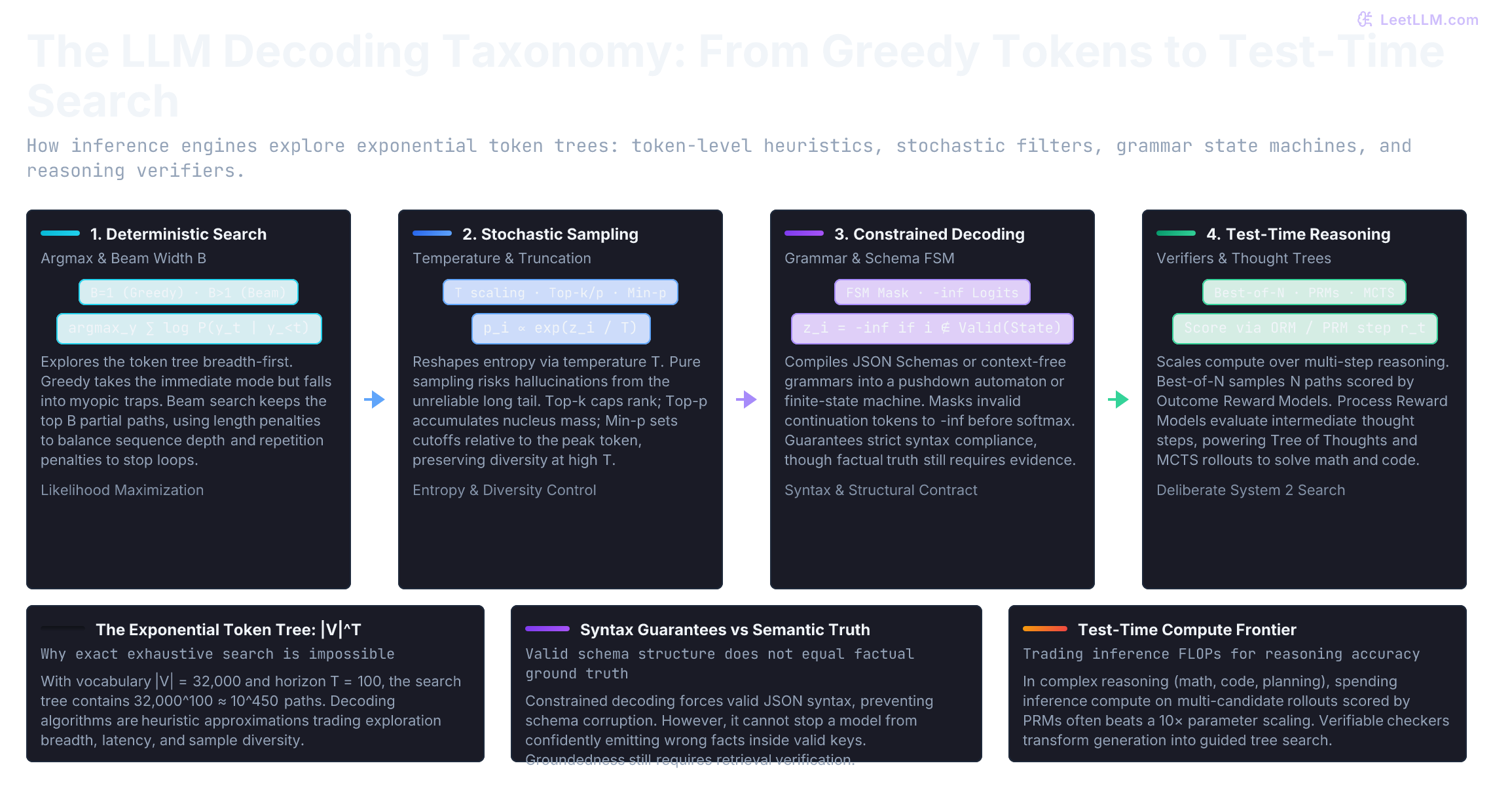
From raw logits to numerically stable probabilities
For clear arithmetic, treat each word below as a single token. Our prompt ends with:
1Evidence: Create a replacement key, deploy it, then revoke the old key.
2Answer: The first rotation step is
Suppose the model outputs these raw prediction scores, called logits, for the immediate next token:
| Token | Logit | Role in rotation runbook |
|---|---|---|
create | 3.0 | Supported by evidence as the initial action. |
revoke | 2.5 | Valid runbook action, but performing it first causes an outage. |
rename | 1.0 | Fluent distractor if account settings leaked into context. |
quota | -1.0 | Irrelevant tail token from an API dashboard. |
Logits aren't probabilities: they're real numbers that can be negative and don't sum to one. Softmax converts unbounded logits into a normalized probability distribution:
Subtracting the maximum logit doesn't alter the output probabilities. Because , the constant factor factors out of both numerator and denominator and cancels cleanly.
This shift prevents exponential overflow when logits grow large, a practical necessity in FP16 and FP32 inference engines.[1] Without it, evaluating crashes floating-point hardware with an overflow exception.
1import numpy as np
2
3tokens = ["create", "revoke", "rename", "quota"]
4logits = [3.0, 2.5, 1.0, -1.0]
5
6def softmax(scores) -> np.ndarray:
7    scores = np.asarray(scores, dtype=np.float64)
8    if scores.ndim != 1 or scores.size == 0:
9        raise ValueError("scores must be a nonempty vector")
10    if np.isnan(scores).any() or np.isposinf(scores).any():
11        raise ValueError("NaN and positive infinity are invalid logits")
12    if not np.isfinite(scores).any():
13        raise ValueError("all tokens are masked")
14    # Negative infinity represents an intentional mask and gets zero weight.
15    weights = np.exp(scores - scores.max())
16    return weights / weights.sum()
17
18probabilities = softmax(logits)
19for token, score, probability in zip(tokens, logits, probabilities):
20    print(f"{token:8} logit={score:>4.1f} probability={probability:.3f}")
21print(f"sum={sum(probabilities):.3f}")1create logit= 3.0 probability=0.568
2revoke logit= 2.5 probability=0.345
3rename logit= 1.0 probability=0.077
4quota logit=-1.0 probability=0.010
5sum=1.000create is the distribution's mode at 0.568. But revoke still holds 0.345 of the total mass: over a third of the probability distribution points to an action that revokes active credentials before new keys are deployed.
Sampling unconstrained from this distribution will trigger production incidents in roughly one out of every three requests.
Numerical stability under extreme ranges
The max shift isn't an optional speed trick. Directly calling exp(1000) overflows standard 64-bit floating-point math, even though the resulting probabilities are mathematically well behaved.
1from math import exp
2
3large_logits = [1000.0, 999.0, 998.0]
4
5try:
6    raw_weights = [exp(score) for score in large_logits]
7    naive = [weight / sum(raw_weights) for weight in raw_weights]
8    print("naive:", naive)
9except OverflowError:
10    print("naive softmax: overflow")
11
12print("stable:", softmax(large_logits).round(3).tolist())
13print("extreme gap:", softmax([0.0, -1000.0]).tolist())
14try:
15    softmax([-np.inf, -np.inf])
16except ValueError as exc:
17 print("rejected:", str(exc))1naive softmax: overflow
2stable: [0.665, 0.245, 0.09]
3extreme gap: [1.0, 0.0]
4rejected: all tokens are maskedThe max subtraction eliminates exponential overflow, but hardware floating-point numbers still have finite precision. An extreme negative gap like exp(-1000) safely underflows to 0.0.
When every token is masked to negative infinity, total probability mass collapses to zero: the decoder must handle that condition explicitly rather than dividing zero by zero.
Deterministic search: greedy myopic traps and beam exploration
After picking a token, the runtime appends it to the prefix and feeds the extended sequence back into the model to predict the subsequent position. Repeating that process builds the autoregressive loop.
In serving runtimes, a key-value (KV) cache retains previous attention keys and values so earlier positions aren't recalculated from scratch.[2] That architecture optimizes inference throughput, but it doesn't choose the token. Selecting tokens remains the responsibility of the decoding algorithm.
Greedy decoding picks the token with the highest logit at every step:
1example_logits = [
2    {"create": 3.0, "revoke": 2.5, "rename": 1.0, "quota": -1.0},
3    {".": 4.0, "then": 1.5, "after": 0.5},
4]
5
6def greedy_token(scores: dict[str, float]) -> str:
7    return max(scores, key=scores.get)
8
9generated = []
10for step, scores in enumerate(example_logits, start=1):
11    chosen = greedy_token(scores)
12    generated.append(chosen)
13    print(f"step {step}: chose {chosen!r} from {len(scores)} candidates")
14
15answer = "The first rotation step is " + " ".join(generated).replace(" .", ".")
16print(answer)1step 1: chose 'create' from 4 candidates
2step 2: chose '.' from 3 candidates
3The first rotation step is create.Greedy generation is completely deterministic. Given identical inputs, hardware, and tie-breaking rules, it always returns the exact same sequence. It requires no hyperparameters, adds zero search overhead, and works well for structured code generation or focused factual extraction.
Yet greedy decoding suffers from a fundamental search failure: the myopic trap. Because greedy search commits irreversibly to the immediate highest-scoring token at step , it can miss globally higher-probability sequences that begin with a slightly lower-scoring first token.
Beam search tracks parallel hypotheses
Beam search mitigates greedy myopia by maintaining a set of active hypotheses, where is the beam width.
At each step, the algorithm:
- Expands all currently retained partial sequences by considering all possible continuations in .
- Computes the cumulative log-probability for each candidate extension: .
- Prunes the pool back to the top highest-scoring paths.
Consider an example where the prompt prefix is You should. Greedy immediately grabs create at step 1 because . But look at what happens at step 2:
| Candidate path | Step 1 prob | Step 2 continuation | Step 2 prob | Joint probability |
|---|---|---|---|---|
create . | 0.40 | . | 0.20 | (Greedy) |
first create | 0.35 | create | 0.70 | (Beam winner) |
revoke . | 0.25 | . | 0.30 | (Pruned) |
Greedy gets trapped with create . at joint probability . A beam search with width retains both create and first through step 1. At step 2, it evaluates the joint paths and discovers first create at : more than triple the joint probability of the greedy choice.
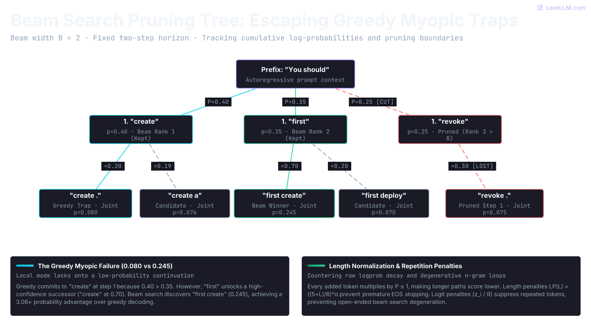
create at step 1 because 0.40 > 0.35, landing on create . at joint score 0.080. Width-2 beam search keeps first alive, unlocking first create at joint score 0.245 (a 3.06× probability advantage). Length normalization and repetition penalties keep longer beams from collapsing into brevity or loops.1from math import exp, isclose, log
2
3first_step = {"create": 0.40, "first": 0.35, "revoke": 0.25}
4second_step = {
5 "create": {".": 0.20, "a": 0.19, "the": 0.18, "your": 0.17, "another": 0.14, "one": 0.12},
6 "first": {"create": 0.70, "deploy": 0.20, "revoke": 0.10},
7 "revoke": {".": 0.30, "the": 0.25, "your": 0.25, "it": 0.20},
8}
9
10def beam_search(distributions, width: int, steps: int):
11 if type(width) is not int or width < 1:
12 raise ValueError("beam width must be a positive integer")
13 beam = [((), 0.0)]
14 for _ in range(steps):
15 candidates = []
16 for prefix, score in beam:
17 probs = distributions[prefix]
18 assert isclose(sum(probs.values()), 1.0)
19 assert all(0 <= p <= 1 for p in probs.values())
20 for token, p in probs.items():
21 if p > 0:
22 candidates.append((prefix + (token,), score + log(p)))
23 beam = sorted(candidates, key=lambda row: row[1], reverse=True)[:width]
24 return beam
25
26tree = {(): first_step, **{(token,): probs for token, probs in second_step.items()}}
27greedy_first = max(first_step, key=first_step.get)
28greedy_second = max(second_step[greedy_first], key=second_step[greedy_first].get)
29greedy_prob = first_step[greedy_first] * second_step[greedy_first][greedy_second]
30
31winner, winner_log_p = beam_search(tree, width=2, steps=2)[0]
32print("greedy:", f"{greedy_first} {greedy_second}", f"probability={greedy_prob:.3f}")
33print("beam: ", " ".join(winner), f"probability={exp(winner_log_p):.3f}")1greedy: create . probability=0.080
2beam: first create probability=0.245Beam search remains an approximate heuristic. Once a prefix falls outside the top hypotheses at any step, the search discards it permanently. Even if that pruned prefix would have unlocked a continuation with probability , beam search can never recover it.
1counterexample = {
2    (): {"A": 0.5, "B": 0.3, "C": 0.2},
3    ("A",): {str(i): 0.1 for i in range(10)},
4    ("B",): {str(i): 0.2 for i in range(5)},
5    ("C",): {"win": 1.0},
6}
7for width in (2, 3):
8    path, score = beam_search(counterexample, width, steps=2)[0]
9 print(f"width={width}: {' '.join(path)} probability={exp(score):.3f}")1width=2: B 0 probability=0.060
2width=3: C win probability=0.200Width prunes branch C at step 1 because . It then settles for B 0 at joint probability 0.060. Expanding width to preserves C, discovering the global optimum C win at joint probability 0.200.
Scaling beam width increases hypothesis coverage, but running concurrent beams multiplies memory footprint and KV-cache storage by .
Length normalization and repetition penalties
Unconstrained beam search encounters two notorious failure modes in production generation: short-sequence bias and degenerative repetition loops.
Length normalization prevents premature termination
Every generated token multiplies the joint probability by a conditional value . In log space, adding non-positive log-probabilities causes cumulative path scores to decay monotonically with sequence length:
A completed two-token answer almost always has a higher raw joint log-probability than an insightful 15-token explanation. Raw beam search is artificially biased toward emitting the end-of-sequence token as early as possible.
To compare sequences of different lengths fairly, we apply a length penalty . Wu et al. developed the Google Neural Machine Translation length penalty:[3]
The exponent tunes length tolerance. At , there is no penalty; at , the score approaches average log-probability per token.[4]
1candidates = [
2    {"text": "create <EOS>", "log_probability": -1.0, "tokens": 2},
3    {"text": "create deploy then revoke <EOS>", "log_probability": -1.6, "tokens": 5},
4]
5
6raw_winner = max(candidates, key=lambda row: row["log_probability"])
7normalized_winner = max(candidates, key=lambda row: row["log_probability"] / row["tokens"])
8
9print("raw winner:               ", raw_winner["text"])
10print("length-normalized winner: ", normalized_winner["text"])
11for row in candidates:
12    average = row["log_probability"] / row["tokens"]
13 print(f"{row['text']:31} raw={row['log_probability']:.3f} average={average:.3f}")1raw winner: create <EOS>
2length-normalized winner: create deploy then revoke <EOS>
3create <EOS> raw=-1.000 average=-0.500
4create deploy then revoke <EOS> raw=-1.600 average=-0.320Raw scoring prefers the terse -1.000 completion. Length normalization divides by token count: -1.600 / 5 = -0.320 beats -1.000 / 2 = -0.500, correctly selecting the complete procedure.
Repetition penalties break self-reinforcing loops
In open-ended tasks like dialogue or report generation, standard beam search frequently degenerates into repetitive loops:
The incident team notified the manager and notified the manager and notified the manager...
Language models attend to their own generated tokens. Once an n-gram repeats, self-attention reinforces that pattern, assigning high conditional probabilities to repeating it again. Maximization-based search greedily exploits this loop.[5]
Keskar et al. introduced a multiplicative logit penalty that discounts any token that has already appeared in the generated prefix:[6]
Dividing positive logits by lowers their probability; multiplying negative logits by pushes them further negative. This penalizes repetition without banning words outright.
1def apply_repetition_penalty(
2    logits: dict[str, float], sequence: list[str], theta: float = 1.2
3) -> dict[str, float]:
4    penalized = dict(logits)
5    for token in set(sequence):
6        if token in penalized:
7            score = penalized[token]
8            penalized[token] = score / theta if score > 0 else score * theta
9    return penalized
10
11step_logits = {"create": 3.0, "deploy": 2.8, "revoke": 2.5}
12print("unpenalized choice:", max(step_logits, key=step_logits.get))
13
14# After 'create' was emitted at step 1, apply repetition penalty:
15penalized = apply_repetition_penalty(step_logits, ["create"], theta=1.2)
16print("penalized 'create' logit:", f"{penalized['create']:.2f}")
17print("penalized choice: ", max(penalized, key=penalized.get))1unpenalized choice: create
2penalized 'create' logit: 2.50
3penalized choice: deployWith , the logit for create drops from 3.0 to 2.50. That demotes create below deploy (2.8), steering the decoder to the next required operation instead of stuttering on the same verb.
Temperature reshapes entropy
Stochastic sampling trades exact log-likelihood maximization for linguistic variety. The first parameter governing this tradeoff is temperature , which scales logits prior to softmax:
- As , the probability distribution collapses into a one-hot vector on the mode . The sampler behaves like greedy search.
- When , probabilities match the model's raw unscaled distribution.
- As , logits are squashed toward zero, converting the distribution into uniform random noise where every token has probability .
We measure the dispersion of the distribution using Shannon entropy: . When using natural logarithms, entropy is expressed in nats. Higher entropy means greater output unpredictability.
1tokens = ["create", "revoke", "rename", "quota"]
2logits = [3.0, 2.5, 1.0, -1.0]
3
4def entropy(probabilities) -> float:
5    positive = np.asarray(probabilities)[np.asarray(probabilities) > 0]
6    return float(-np.sum(positive * np.log(positive)))
7
8for temperature in (0.5, 1.0, 2.0):
9    probabilities = softmax([score / temperature for score in logits])
10    table = dict(zip(tokens, probabilities))
11    print(
12        f"T={temperature:.1f}: create={table['create']:.3f} "
13        f"quota={table['quota']:.3f} entropy={entropy(probabilities):.3f}"
14 )1T=0.5: create=0.721 quota=0.000 entropy=0.647
2T=1.0: create=0.568 quota=0.010 entropy=0.933
3T=2.0: create=0.438 quota=0.059 entropy=1.190At , entropy falls to nats and create claims of the probability mass. At , entropy rises to nats: the irrelevant tail token quota jumps from to nearly .
Lowering temperature sharpens the distribution, but it doesn't remove bad tokens mathematically. As long as , every token with a finite logit retains non-zero probability.
Does setting temperature to 0.2 eliminate the risk of sampling an unsupported tail token?
Answer
No. Temperature compresses logit gaps but leaves every finite token with positive probability. Even at T = 0.2, tail tokens retain non-zero mass. To guarantee that low-probability candidates cannot be sampled, you must use truncation filters or grammar constraints.
Seeding and production reproducibility
Sampling draws random tokens according to model probabilities. In local development, passing a fixed random seed allows repeatable draws from a static distribution:
1from random import Random
2
3tokens = ["create", "revoke", "rename", "quota"]
4probabilities = [0.568, 0.345, 0.077, 0.010]
5
6def draw_sequence(seed: int, length: int = 8) -> list[str]:
7    rng = Random(seed)
8    return rng.choices(tokens, weights=probabilities, k=length)
9
10for seed in (7, 7, 21):
11 print(f"seed={seed}: {' '.join(draw_sequence(seed))}")1seed=7: create create revoke create create create create create
2seed=7: create create revoke create create create create create
3seed=21: create revoke revoke create create revoke revoke createLocal seeds ensure test determinism. But in production GPU clusters, exact byte-for-byte reproducibility is difficult to guarantee.
Parallel matrix multiplications (such as cuBLAS GEMM or FlashAttention) perform floating-point additions across distributed GPU threads. Because floating-point addition is non-associative, small variations in dynamic request batching or CUDA thread scheduling alter intermediate sums slightly. Those micro-variations can flip borderline logits and steer sampling onto entirely different paths.
Hosted model providers also update inference backends and quantization layers over time. For example, Anthropic's Claude Sonnet 5 rejects custom temperature, top_p, and top_k parameters entirely, returning a 400 Bad Request if developers attempt to override default values.[7]
Production evaluation harnesses must log model version hashes, prompt snapshots, decoder parameters, and vendor response headers alongside each generated answer.
Truncating the long tail: Top-k, Top-p, and Min-p
Unconstrained sampling from the entire vocabulary inevitably pulls from what Holtzman et al. call the unreliable tail.[5] Even if an absurd token has a tiny probability of , over an answer of 500 tokens the probability of drawing at least one tail token is:
To prevent tail pollution, inference engines truncate the vocabulary before drawing tokens.
Top-k truncation: fixed rank cutoff
Top-k sampling retains only the highest-probability tokens, setting the probability of all other tokens to zero and renormalizing the remaining mass:[8]
1from math import isclose, isfinite
2
3peaked = {"create": 0.568, "revoke": 0.345, "rename": 0.077, "quota": 0.010}
4
5def ranked_distribution(probabilities: dict[str, float]) -> list[tuple[str, float]]:
6    values = list(probabilities.values())
7    if not values or any(not isfinite(p) or p < 0 for p in values):
8        raise ValueError("probabilities must be finite and nonnegative")
9    if not isclose(sum(values), 1.0, rel_tol=1e-12, abs_tol=1e-12):
10        raise ValueError("probabilities must sum to one")
11    return sorted(
12        ((token, p) for token, p in probabilities.items() if p > 0),
13        key=lambda row: row[1], reverse=True,
14    )
15
16def top_k(probabilities: dict[str, float], k: int) -> list[tuple[str, float]]:
17    if type(k) is not int or k < 1:
18        raise ValueError("k must be a positive integer")
19    ranked = ranked_distribution(probabilities)[:k]
20    retained_mass = sum(prob for _, prob in ranked)
21    return [(token, prob / retained_mass) for token, prob in ranked]
22
23for token, prob in top_k(peaked, k=2):
24 print(f"{token:8} renormalized={prob:.3f}")1create renormalized=0.622
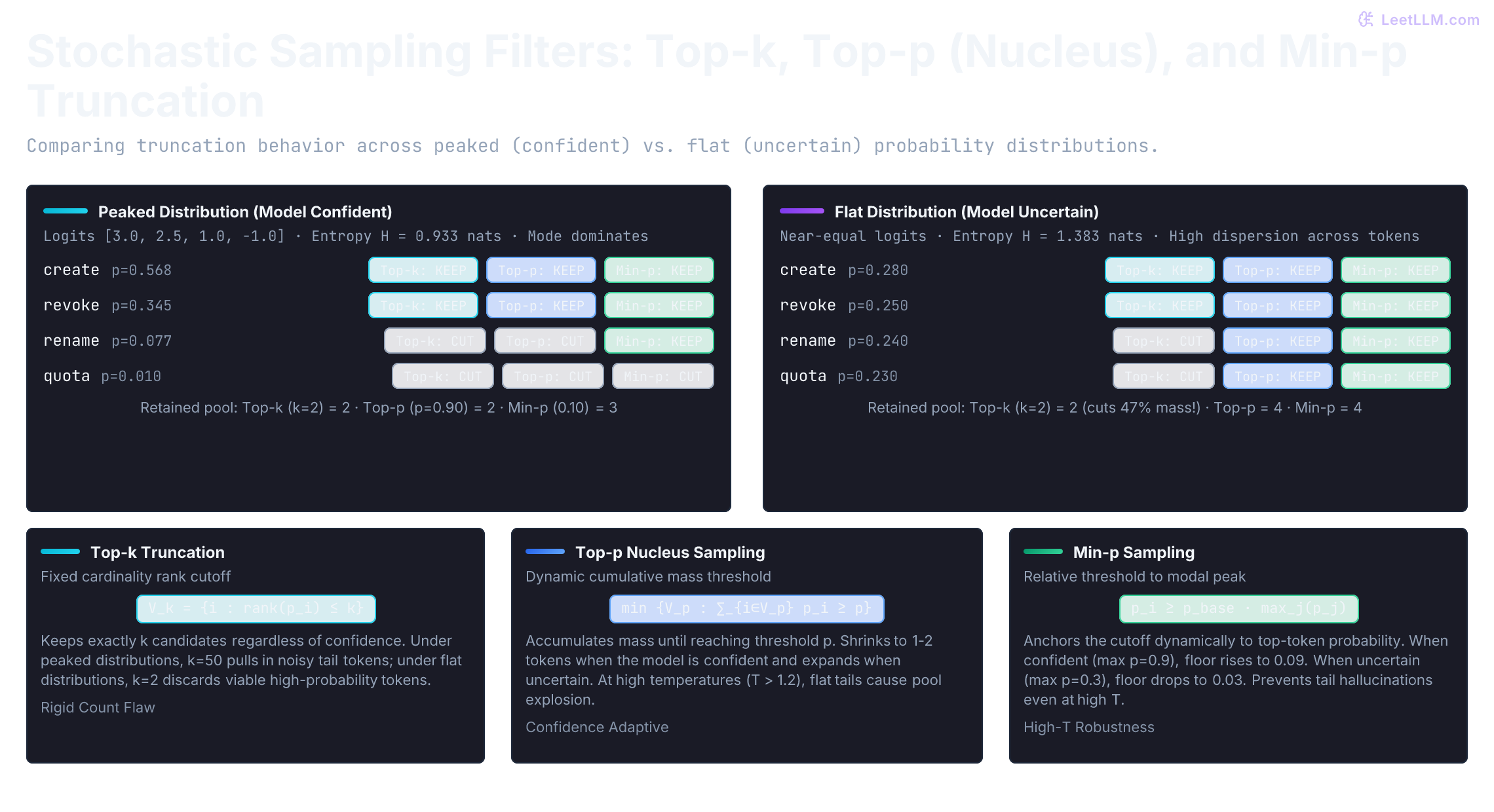
2revoke renormalized=0.378Top-k sampling has a major structural flaw: fixed cardinality.
When the model is confident and the distribution is steep (for instance, completing The capital of France is), the single correct token might hold of the mass. A setting of forces the sampler to keep 49 garbage tokens.
Conversely, when the distribution is flat because many synonyms are equally valid, arbitrarily cuts off good candidates that happen to rank 51st.
Top-p (Nucleus) sampling: dynamic cumulative thresholding
Top-p sampling, or nucleus sampling, solves the fixed-cardinality problem by accumulating mass. It selects the smallest set of ranked tokens whose cumulative probability reaches a threshold :[5]
1def nucleus(probabilities: dict[str, float], threshold: float) -> list[str]:
2    if not isfinite(threshold) or not 0 < threshold <= 1:
3        raise ValueError("top-p threshold must be in (0, 1]")
4    ranked = ranked_distribution(probabilities)
5    if threshold == 1:
6        return [token for token, _ in ranked]
7    kept = []
8    cumulative = 0.0
9    for token, prob in ranked:
10        kept.append(token)
11        cumulative += prob
12        if cumulative >= threshold:
13            break
14    return kept
15
16peaked = {"create": 0.568, "revoke": 0.345, "rename": 0.077, "quota": 0.010}
17flat = {"create": 0.28, "revoke": 0.25, "rename": 0.24, "quota": 0.23}
18
19print("peaked p=0.90:", nucleus(peaked, 0.90))
20print("flat p=0.90:", nucleus(flat, 0.90))1peaked p=0.90: ['create', 'revoke']
2flat p=0.90: ['create', 'revoke', 'rename', 'quota']At , Top-p keeps only 2 tokens for the peaked distribution (). For the flat distribution, it dynamically expands to keep all 4 tokens. Top-p adapts candidate pool size to the model's certainty.
Min-p sampling: relative probability filtering
Top-p works well at moderate temperatures (), but it struggles at higher temperatures (). High temperatures flatten the entire vocabulary tail. Because hundreds of near-zero probabilities accumulate slowly, reaching forces Top-p to retain a massive pool of noisy tail tokens, triggering syntactic degeneration.
Min-p sampling sets its truncation threshold relative to the top candidate's probability.[9] Instead of fixing rank or cumulative mass , it keeps only tokens whose probability is at least a fraction of the maximum token's probability:
1def min_p(probabilities: dict[str, float], base_threshold: float) -> list[str]:
2    if not isfinite(base_threshold) or not 0 <= base_threshold <= 1:
3        raise ValueError("min-p threshold must be in [0, 1]")
4    ranked = ranked_distribution(probabilities)
5    max_p = ranked[0][1]
6    cutoff = base_threshold * max_p
7    return [token for token, p in ranked if p >= cutoff]
8
9peaked = {"create": 0.568, "revoke": 0.345, "rename": 0.077, "quota": 0.010}
10flat = {"create": 0.28, "revoke": 0.25, "rename": 0.24, "quota": 0.23}
11
12print("peaked min-p=0.10:", min_p(peaked, 0.10))
13print("flat min-p=0.10:", min_p(flat, 0.10))1peaked min-p=0.10: ['create', 'revoke', 'rename']
2flat min-p=0.10: ['create', 'revoke', 'rename', 'quota']Under the peaked distribution, the top token is create at 0.568. With , the absolute cutoff is . rename () survives, but quota () is discarded.
Under the flat distribution, the top token is 0.28, establishing a cutoff of . All four tokens easily clear that bar.
Min-p scales its cutoff with the model's confidence. When the model is certain (), the cutoff jumps to , aggressively pruning the tail. When the model is uncertain (), the cutoff falls to , preserving healthy exploration.
Hugging Face includes native support for min_p directly in GenerationConfig.[4]
Boundary cases in filter implementations
Production filter implementations must handle boundary conditions predictably:
1boundary = {"create": 0.5, "revoke": 0.25, "rename": 0.25, "quota": 0.0}
2print("top-k k=2: ", [token for token, _ in top_k(boundary, 2)])
3print("top-p p=.75:", nucleus(boundary, 0.75))
4print("top-p p=1:  ", nucleus(boundary, 1.0))
5print("min-p=.5:   ", min_p(boundary, 0.5))
6print("min-p=1:    ", min_p({"create": 0.5, "revoke": 0.5}, 1.0))
7
8for label, call in [
9    ("k=0", lambda: top_k(boundary, 0)),
10    ("p=0", lambda: nucleus(boundary, 0)),
11    ("zero mass", lambda: min_p({"create": 0.0}, 0.1)),
12]:
13    try:
14        call()
15    except ValueError as exc:
16 print(label, "REJECT", str(exc))1top-k k=2: ['create', 'revoke']
2top-p p=.75: ['create', 'revoke']
3top-p p=1: ['create', 'revoke', 'rename']
4min-p=.5: ['create', 'revoke', 'rename']
5min-p=1: ['create', 'revoke']
6k=0 REJECT k must be a positive integer
7p=0 REJECT top-p threshold must be in (0, 1]
8zero mass REJECT probabilities must sum to oneThese checks protect against silent generation failures. In production pipelines, apply temperature scaling before running truncation filters, and renormalize surviving candidates before drawing.

Grammar-constrained decoding: syntax enforcement versus semantic truth
Production applications frequently require models to produce structured outputs: valid JSON, strict enum values, or executable SQL. Left unconstrained, a model might emit valid JSON for 200 tokens and then break the parser with a trailing comma or unescaped quote.
Constrained decoding prevents syntax violations by applying a formal grammar (Context-Free Grammar, JSON Schema, or Regular Expression) directly to the decoding loop.[10][11][12]
The grammar compiler compiles the schema into a Finite-State Machine (FSM) or pushdown automaton. At each decoding step:
- The FSM inspects its current state and identifies the set of allowable next characters or bytes.
- The engine maps those allowed transitions against the tokenizer vocabulary.
- Any token that would transition the output into an invalid state has its logit forced to prior to softmax:
Because masked tokens receive an exponent of zero (), their probability drops to zero. The model is mathematically incapable of emitting a syntax error.
1logits = {"quota": 6.0, "revoke": 4.0, "create": 3.0, "rename": 2.0}
2schema_values = {"create", "revoke", "rename"}
3supported_by_guide = {"create"}
4
5def constrained_greedy(scores: dict[str, float], allowed: set[str]) -> str:
6    candidates = {token: score for token, score in scores.items() if token in allowed}
7    if not candidates:
8        raise ValueError("constraint removed every token")
9    return max(candidates, key=candidates.get)
10
11print("unconstrained:     ", max(logits, key=logits.get))
12print("schema-only:       ", constrained_greedy(logits, schema_values))
13print("evidence-supported:", constrained_greedy(logits, supported_by_guide))1unconstrained: quota
2schema-only: revoke
3evidence-supported: createNotice the clear distinction between the second and third lines:
- Unconstrained decoding picks
quotabecause it has the highest logit (6.0). - Schema-constrained decoding masks
quota, but picksrevoke(4.0) becauserevokeis a valid enum field in the JSON Schema. - Evidence-supported decoding picks
createbecause external validation confirmed it as the correct initial runbook step.
This illustrates the core boundary of constrained decoding: syntax enforcement is not semantic verification.[13]
An engine using OpenAI Structured Outputs or Outlines will guarantee valid JSON format with 100% syntactic reliability. But if the model chooses to hallucinate incorrect data inside a syntactically valid field, grammar masking can't detect the error. Verifying factual accuracy requires external validation or reasoning search.
Test-time search and reasoning: verifiers and thought trees
Recent advances in reasoning models (OpenAI o1/o3, DeepSeek-R1) shift computational effort from training time to inference time. Snell et al. demonstrated that scaling inference compute via test-time search can outperform scaling pretraining compute by 10× on complex reasoning tasks.[14]
Instead of searching blindly across raw token spaces, test-time search operates across complete trajectories or discrete reasoning steps.
Best-of-N rejection sampling with Outcome Reward Models
In Best-of-N sampling, the engine samples complete, independent candidate answers at temperature . An Outcome Reward Model (ORM) scores each finished sequence, and the highest-scoring candidate is selected as the final answer:[15]
Alternatively, in domains with verifiable ground truth (such as competitive programming or mathematical proofs), an automated checker (unit test runner or formal theorem prover) evaluates candidates directly.
Process Reward Models catch intermediate reasoning failures
While ORMs evaluate the final answer, they suffer from a severe credit assignment problem on multi-step reasoning.[16] A model might follow flawed logic for 10 steps, make an offsetting arithmetic mistake, and stumble upon the correct final answer (a false positive). Conversely, a model might execute 10 brilliant deductive steps, make a minor typo on step 11, and receive a score of zero (a false negative).
Process Reward Models (PRMs) evaluate each intermediate reasoning step individually:
1candidates = [
2    {
3        "id": "plan_A",
4        "steps": ["Create replacement key", "Deploy key to cluster", "Revoke old key"],
5        "prm_steps": [0.95, 0.92, 0.98],
6        "orm_score": 0.96,
7    },
8    {
9        "id": "plan_B",
10        "steps": ["Revoke old key immediately", "Create replacement key", "Deploy key to cluster"],
11        "prm_steps": [0.05, 0.90, 0.92],
12        "orm_score": 0.72,
13    },
14]
15
16def prm_min_score(traj: dict) -> float:
17    return min(traj["prm_steps"])
18
19orm_best = max(candidates, key=lambda t: t["orm_score"])
20prm_best = max(candidates, key=prm_min_score)
21
22print(f"ORM best: {orm_best['id']} (score={orm_best['orm_score']:.2f})")
23print(f"PRM best: {prm_best['id']} (min_step={prm_min_score(prm_best):.2f})")
24for t in candidates:
25 print(f"{t['id']}: ORM={t['orm_score']:.2f} PRM_min={prm_min_score(t):.2f} first_step={t['steps'][0]!r}")1ORM best: plan_A (score=0.96)
2PRM best: plan_A (min_step=0.92)
3plan_A: ORM=0.96 PRM_min=0.92 first_step='Create replacement key'
4plan_B: ORM=0.72 PRM_min=0.05 first_step='Revoke old key immediately'Look closely at plan_B: step 1 revokes the old key before deploying a replacement. That immediately causes an active production outage.
A naive ORM that only evaluates whether all three rotation actions were mentioned scores plan_B at 0.72. But the PRM immediately catches the operational failure on step 1, scoring it at 0.05 and disqualifying the dangerous plan.
Tree of Thoughts and Monte Carlo Tree Search
Rather than sampling flat complete trajectories, advanced inference runtimes treat reasoning as search over a tree of thoughts.[17]
Each node in the tree represents a partial reasoning state (a thought step or sub-goal). The search engine uses PRM step scores or heuristic value functions to:
- Expand: Propose candidate next reasoning thoughts.
- Evaluate: Score the validity of each thought using a PRM.
- Backtrack: When all extensions from a reasoning branch yield poor scores (), backtrack to a parent node and explore alternative deductions.
- Roll out: Use Monte Carlo Tree Search (MCTS) to simulate continuations toward the final solution.[18]
By operating at the thought level rather than the token level, test-time search navigates the exponential token tree with deliberate, System 2 problem solving.
Speculative decoding: lossless serving optimization
Deterministic search, stochastic sampling, and test-time reasoning all alter the text the model outputs. Speculative decoding solves a completely different challenge: reducing inference latency without changing the output distribution by even a single bit.[19]
Standard autoregressive decoding requires one forward pass of the multi-billion-parameter target model per generated token. Because memory bandwidth limits GPU processing when generating tokens one at a time, execution arithmetic intensity is low.
Speculative decoding pairs the large target model with a small, lightweight draft model :
- Draft phase: The small draft model autoregressively proposes a burst of candidate tokens quickly.
- Verification phase: The large target model processes all proposed tokens in a single parallel forward pass, evaluating their exact conditional probabilities: .
- Modified rejection sampling: For each draft token , if the target probability (where is the draft probability), the token is accepted. If , the token is accepted with probability .
- Correction: If a token is rejected at index , the remaining draft tokens are discarded. The target model draws a replacement token from the adjusted residual distribution without requiring another forward pass.
This verification math proves that the output text matches the exact sampling distribution of the large target model.
Speculative decoding provides a 2× to 3× wall-clock speedup on memory-bound workloads, but it doesn't change model behavior or fix factual errors.
| Technique | Primary operational objective | Changes output distribution? |
|---|---|---|
| Greedy Search | Low-latency local likelihood maximization | Yes (mode collapse) |
| Beam Search | Sequence-level joint likelihood exploration | Yes (maximization bias) |
| Temperature / Top-p / Min-p | Tail suppression and diversity control | Yes (entropy modulation) |
| Grammar-Constrained FSM | 100% schema and syntax validity | Yes (hard negative masks) |
| Test-Time Search (PRM / MCTS) | Multi-step reasoning and verification | Yes (trajectory reranking) |
| Exact Speculative Decoding | Serving throughput and latency acceleration | No (lossless equivalence) |
Production generation audits and offline evaluation
When tweaking retrieval algorithms, prompt templates, or inference engines, teams frequently alter decoding configurations simultaneously. If retrieval embeddings and temperature change in the same deployment, you can't tell which change caused an answer regression.
A generation audit record must capture:
- Prompt hash, model identifier, and runtime build version.
- Retrieval evidence snapshot ID and document chunks.
- Decoding configuration: temperature, top-k, top-p, min-p, beam width, and length penalty.
- Repetition penalty and grammar FSM schema version.
- Random seed and engine stop reason (e.g.
stop_token,length_limit). - Ground truth verification judgments.
To audit decoder mechanics, run controlled simulations against fixed distributions before conducting full user-facing experiments.
1from math import exp
2from random import Random
3
4def distribution(temperature):
5    if not isfinite(temperature) or temperature <= 0:
6        raise ValueError("temperature must be finite and positive")
7    scores = dict(create=3.0, revoke=2.5, rename=1.0, quota=-1.0)
8    weights = {token: exp((z - max(scores.values())) / temperature) for token, z in scores.items()}
9    total = sum(weights.values())
10    return {token: weight / total for token, weight in weights.items()}
11
12base = distribution(1.0)
13kept = nucleus(base, 0.9)
14retained_mass = sum(base[token] for token in kept)
15policies = {
16    "greedy":     {max(base, key=base.get): 1.0},
17    "sample T=2": distribution(2.0),
18    "top-p p=.9": {token: base[token] / retained_mass for token in kept},
19}
20
21for label, probabilities in policies.items():
22    rng = Random(7)
23    outputs = rng.choices(list(probabilities), weights=list(probabilities.values()), k=2000)
24    observed = outputs.count("create") / len(outputs)
25 print(f"{label:12} expected={probabilities.get('create', 0):.3f} observed={observed:.3f}")1greedy expected=1.000 observed=1.000
2sample T=2 expected=0.438 observed=0.457
3top-p p=.9 expected=0.622 observed=0.621Greedy outputs the supported action create 100% of the time. Top-p at retains both create and revoke, selecting create in of draws and emitting the dangerous revoke in roughly . Sampling at drops the supported action rate to .
Decoders only manipulate scores: they don't understand infrastructure safety. If the model had assigned a higher logit to revoke, greedy decoding would execute the dangerous step every single time. Real-world reliability requires pairing appropriate decoding algorithms with grounded evidence retrieval and verified system testing.