Personalize this lesson
Adapt explanations and teaching visuals to your background and preferred voice.
Over half of published reinforcement learning and deep learning papers fail to replicate when independent teams rerun their code. As Henderson and colleagues demonstrated across standard benchmarks,[1] researchers routinely sweep dozens of random seeds, pluck out the single best training curve that happened to roll lucky exploratory transitions, and present that smooth outlier as an algorithmic breakthrough. Couple that random seed lottery with floating package versions (numpy>=1.24, torch), non-deterministic GPU kernel dispatches,[2] and evaluation metrics that accidentally score agents on auxiliary training rewards rather than true task return, and the claimed performance gain quickly collapses into statistical noise.
When you evaluate a research paper or propose a candidate algorithm for production, you can't rely on cherry-picked runs or optimistic blog posts. You need an ironclad experimental protocol: a pre-locked mathematical contract, paired random seed trials that isolate algorithmic treatment effects from initialization noise, non-parametric uncertainty estimates that don't falsely assume Gaussian returns, and cryptographic manifests that guarantee deterministic rerun invariance.
This study builds that complete, auditable research workflow around a classic question from reinforcement learning theory: does potential-based reward shaping accelerate early goal-reaching in a stochastic corridor without degrading the agent's final greedy policy under the true environment reward?
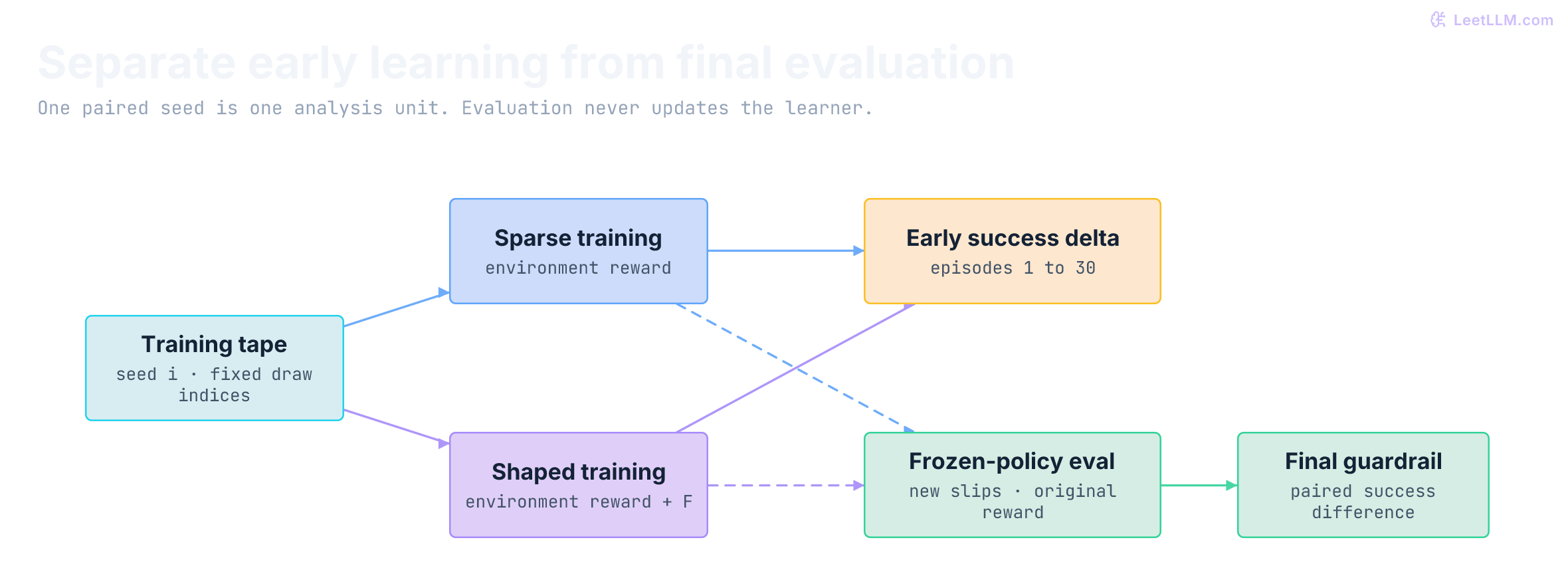
The scope stays deliberately narrow and fully public-safe. The environment reward never changes, and final evaluation never touches the shaping bonus. Everything runs locally with synthetic transitions and NumPy, so no private logs, live users, paid APIs, or specialized hardware enter the study.
This chapter contains a worked run whose results are already known, not evidence that its plan was independently preregistered. Repeating seeds 0 through 23 checks repeatability. For your own confirmatory study, finish pilot debugging, freeze the design, and reserve a new untouched seed set before inspecting results.
Read the claim before building the simulator
The first implementation decision is whether the source contains one claim small enough to test honestly. Start with Ng, Harada, and Russell's paper on policy invariance under reward transformations.[3] Its main claim is precise enough for a small simulator: a potential-based shaping reward can guide learning while preserving optimal policies under the theorem's assumptions.
Don't begin by reproducing every table or proof. Keshav's three-pass reading method gives a practical order: classify the paper, inspect its evidence, then reconstruct the part you plan to test.[4] That order keeps an attractive equation from turning into an unbounded reproduction project.
Use this triage card while reading. Fill it with page or section pointers so a reviewer can trace your interpretation back to source text.
| Triage field | Corridor-study note |
|---|---|
| problem | sparse rewards provide little learning signal before goal completion |
| paper claim | potential-based shaping preserves optimal policies under stated assumptions |
| equation to implement | |
| smallest test | seven-state corridor with tabular Q-learning |
| theorem assumptions to check | same discounted Markov decision process, bounded potential, correct terminal handling |
| measurement control | final evaluation uses original environment reward |
| evidence you can reproduce | learning speed across fixed simulator seeds |
| claim you can't make | the method improves deep RL or deployed agents |
First pass: classify the claim
Keshav's first pass is a short classification scan, not an evidence audit. Read the title, abstract, and introduction; skim section headings; read the conclusion; glance at the references. Don't study the figures yet.
Write one sentence for the problem, method, comparison, and claimed result. If those sentences stay vague, the study isn't ready to design.
For this paper, the method isn't "add helpful rewards." It derives a transition reward from a potential function. That distinction separates the policy-invariance theorem from arbitrary bonuses that can change which policy is optimal.
Stop the first pass with a scope decision: reproduce, extend, or decline. This capstone performs a small empirical check of one implication and adds an uncertainty-focused artifact. It doesn't attempt a full paper reproduction.
Second pass: inspect evidence and assumptions
Now inspect the figures, axes, and error bars, then read the equation, experimental setup, and failure caveats. First write down what stays constant, what changes, and what the paper measures.
Missing implementation detail belongs in an assumptions log, not in a silent guess.
Pay close attention to evaluation reward. A candidate trained with shaped reward can look better if its score includes the extra training bonus. Compare both learned policies using the original environment reward or you have changed the measurement.
Record every adaptation. The corridor, Q-learning hyperparameters, action-slip probability, seed budget, and bootstrap rule are capstone choices rather than claims copied from the paper.
Third pass: reconstruct the test
Explain the shaping equation without looking. Then rebuild the smallest environment where moving toward a goal changes potential. Predict what should happen to early learning and final policy before running code.
Then challenge the design. Could the candidate receive more steps, a friendlier random stream, or an easier evaluation? Could a single lucky seed drive the mean? Every plausible shortcut becomes a control, ablation, or stated limitation.
Finish paper_triage.md with three labels: supported by source, study adaptation, and unresolved. That file prevents a plausible implementation detail from turning into a misattributed paper claim.
Turn curiosity into a falsifiable contract
The triage card names a paper claim and a smallest test. It still doesn't say which observation would count against the idea. "Does reward shaping help agents learn?" is too broad because it leaves the agent, environment, shaping rule, metric, sample, and outcome undefined.
A falsifiable hypothesis names an observation that can contradict it. Narrow scope makes the capstone stronger: every noun can become a file, parameter, table column, or assertion.
Use this research question:
In a stochastic seven-state corridor, does potential-based shaping increase tabular Q-learning's first-30-episode goal-reaching rate versus sparse reward, while keeping final greedy-policy success unchanged under original reward?
Lock the contract before inspecting confirmatory results:
| Contract field | Locked value |
|---|---|
| unit of analysis | one paired simulator seed |
| baseline | tabular Q-learning with sparse terminal reward |
| candidate | same Q-learning plus potential-based shaping during training |
| primary metric | first-30-episode success-rate difference, shaped minus sparse |
| uncertainty | 90% paired bootstrap interval over seed differences |
| minimum useful effect | mean paired difference at least +0.10 |
| final-policy guardrail | observed mean and 90% paired interval stay within [-0.02, +0.02] |
| worked sample | seeds 0 through 23; reserve new seeds for a new confirmatory study |
| stopping rule | run all 24 seed pairs |
State the expected result
Prediction comes before output. A distance-based potential supplies feedback before the first goal, so improved early goal-reaching is a plausible hypothesis. Policy-invariance theory concerns optimal policies, not the policies produced by 80 finite training episodes. Similar final greedy success is an empirical expectation to check, not a consequence guaranteed by the theorem.[3]
That expectation isn't permission to hide a miss. It gives reviewers a record of what you believed before seeing confirmatory values. Exploratory explanations can follow, but they need an explicit label.
Write this expected pattern in study_plan.md before running seeds 0 through 23:
- positive early paired difference
- interval above zero
- near-zero final difference
- timestamp or immutable commit for locked plan
A commit makes later edits visible, but it isn't equivalent to independent preregistration. For formal work, register hypotheses, variables, tests, decision criteria, and exclusions in a timestamped read-only system before collecting confirmatory results.[5]
Write the rejection rule
Support the capstone's narrow claim only if the mean early difference is at least +0.10 and the 90% interval's lower bound is above zero. Also require the final-policy guardrail.
Withhold support for the study claim when either requirement fails. A mean of +0.09 is below the declared point-estimate threshold even if its interval is positive. A mean of +0.20 also fails if final original-reward performance shifts beyond the guardrail. This rule doesn't establish an effect of at least +0.10 with 90% confidence: that stronger claim would require the interval's lower bound to clear +0.10.
"Inconclusive" can be accurate when interval width leaves multiple practical interpretations. Keep that label distinct from "no effect" and from "the candidate is worse."
Keep the study public-safe
Small research work still needs a data and authority boundary. Synthetic data removes many privacy risks, but a public repository can still leak credentials, copied code, or outputs from proprietary environments. Decide that boundary before collecting artifacts.
The corridor generator owns every transition. It doesn't imitate a customer, scrape a service, call an external model, or exercise a live agent. A run is shareable because its complete input is a tiny configuration plus a pseudorandom seed.
Add this boundary to the README before code:
| Surface | Included | Excluded |
|---|---|---|
| data | generated corridor transitions | user messages, production logs, private datasets |
| compute | local CPU and NumPy | remote model APIs, paid accelerators |
| actions | left/right in simulator | browser, shell, account, or network actions |
| outputs | metrics, tables, plots, manifests | secrets, identifiers, raw third-party content |
| claim | this simulator and implementation | human behavior, robotics, deployed-agent safety |
Run a secret scanner before publishing. Review generated files for machine paths and usernames. Use an open license only for code and assets you have authority to release.
Build the smallest controlled environment
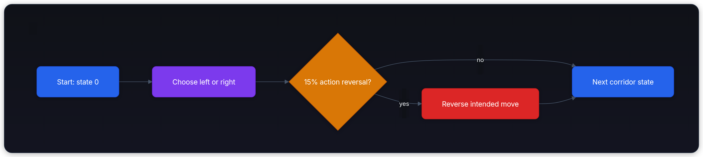
The corridor has states 0 through 6. Every episode starts at 0; reaching 6 yields environment reward 1; every other transition yields 0. An intended action reverses with probability 0.15, and an episode ends after 12 steps.
Write the environment contract before writing the agent. Otherwise a reward, reset, or ending-condition change can enter one arm unnoticed and look like a learning effect.
| Environment field | Locked contract |
|---|---|
| observation | integer state in {0, 1, ..., 6} |
| actions | 0 = left, 1 = right |
| reset | return state 0; select pre-generated tape by seed |
| transition | move one cell, clamp at endpoints, reverse intended move on a 0.15 slip |
| reward | 1 on first arrival at state 6; otherwise 0 |
| terminated | agent reaches state 6 |
| truncated | 12 steps elapse without reaching goal |
| random inputs | exploration, action, tie-break, and slip draws indexed by seed, episode, and step |
| logged output | state, intended action, realized move, environment reward, termination reason |
terminated means the task reached the goal. truncated means an external rollout budget ended collection. The learner estimates discounted return in an underlying task without that 12-step deadline; it still bootstraps at a timeout, but not at the true terminal goal. Our reported success metric is instead goal-reaching within 12 steps. These are related objectives, not identical ones.
If the deadline were part of the task itself, remaining time would belong in the state and deadline expiry would be terminal. Don't silently switch between these formulations.[6] The compact script records episode success and step counts; a full capstone should also retain diagnostic transition traces.
Treating a timeout as terminal success, or bootstrapping through a true terminal, changes the learning target.
Tabular Q-learning stores one value for each state-action pair. During training it moves the chosen action toward observed reward plus the best estimated next-state value. That's the off-policy update from that earlier lesson.[7]
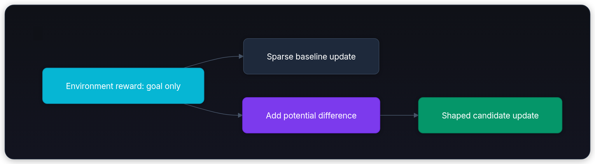
The first diagram follows one environment transition, including the 15% action reversal. Both arms then read the same environment reward; only the candidate receives a training-only potential difference before its update. Final evaluation reads the original reward branch for both arms. Keep that split visible while reading the equations.
Define distance potential as:
States nearer the goal have a larger potential. Candidate training adds:
With discount 0.95, a step toward the goal usually produces a positive shaping signal. A step away usually produces a negative one. Check that on the first two cells before running the 24-seed study. and , so a right move from the start yields , while the reverse move yields .
The environment reward hasn't changed; only candidate training receives . That is the boundary the final evaluation must preserve.
The reason this particular bonus preserves the discounted objective is telescoping. For a trajectory of length :
At the goal, , so every completed trajectory from state 0 receives the same total discounted addition, . A bounded potential also makes the final term vanish in the infinite-horizon discounted limit. At an artificial timeout, the remaining term generally isn't zero. That's why terminal potential and timeout bootstrapping matter; merely writing the equation isn't enough.[3]
The snippet below is the contract for that one transition. It uses the Python standard library so you can verify the arithmetic without NumPy.
1GAMMA = 0.95
2GOAL = 6
3
4def potential(state: int) -> float:
5    return -(GOAL - state) / GOAL
6
7def shaping(state: int, next_state: int) -> float:
8    return GAMMA * potential(next_state) - potential(state)
9
10toward = shaping(0, 1)
11away = shaping(1, 0)
12assert potential(0) == -1
13assert abs(potential(1) - (-5 / 6)) < 1e-12
14assert toward > 0
15assert away < 0
16print(f"Phi(0)={potential(0):.3f}  Phi(1)={potential(1):.3f}")
17print(f"F(0->1)={toward:+.3f}")
18print(f"F(1->0)={away:+.3f}")
19
20# Two completed trajectories take different lengths but get the same addition.
21for path in ([0, 1, 2, 3, 4, 5, 6], [0, 1, 0, 1, 2, 3, 4, 5, 6]):
22    bonus = sum(GAMMA**t * shaping(s, n) for t, (s, n) in enumerate(zip(path, path[1:])))
23    assert abs(bonus - 1.0) < 1e-12
24print("Completed-path discounted bonus: +1.000 for both paths")1Phi(0)=-1.000 Phi(1)=-0.833
2F(0->1)=+0.208
3F(1->0)=-0.117
4Completed-path discounted bonus: +1.000 for both pathsThe comparison table records what stayed paired and what was allowed to differ:
| Component | Sparse baseline | Shaped candidate |
|---|---|---|
| states and actions | identical | identical |
| slip tape | paired | paired |
| Q-learning update | identical | identical |
| environment reward | goal only | goal only |
| training-only addition | none | |
| final evaluation reward | goal only | goal only |
Now the two arms differ in one intended place: the candidate's training update. Controls and paired randomness can test whether that boundary held in code.
Make randomness and controls explicit
Reinforcement learning measurements can vary wildly with random seeds, environment randomness, codebase differences, and hyperparameters. Henderson and colleagues showed that two runs of the same algorithm differing only by random seed can look like two completely different algorithms.[1] Treat the random stream as part of the formal experimental design, not as an invisible background detail.
The paired seed trial protocol
In a standard, unpaired trial, baseline runs on one set of random seeds while candidate runs on another independent set. If is baseline performance and is candidate performance, the variance of the difference between sample means is:
In a stochastic environment, random seed noise (unlucky action slips or cold exploration streaks) inflates both and . You're left with a wide, noisy confidence interval that requires hundreds of runs to resolve.
In a paired seed trial, every seed feeds the exact same sequence of pseudo-random draws to both arms. Because both arms experience the exact same environment transitions for that seed, we compute the paired difference for each seed:
The variance of the sample mean paired difference is:
When seed rolls an unlucky sequence of four slips in a row, both the sparse baseline and the shaped candidate suffer that exact same environmental penalty. That shared difficulty induces a positive covariance between the two arms (). The term actively subtracts out common environmental noise, shrinking estimator variance and tightening the resulting confidence interval without demanding an expensive seed budget.
Synchronizing randomness with a 2D tape
Pairing sounds simple in theory, but naive implementations break it immediately. In reinforcement learning, episode length is dynamic. If the shaped candidate reaches the goal in 4 steps while the sparse baseline wanders for 12 steps, a single sequential random number generator will fall out of sync after episode 0. The shaped arm would draw from PRNG offset 4 on episode 1, while the baseline would draw from PRNG offset 12! From episode 1 onwards, the arms receive completely uncorrelated random numbers.
To keep the arms strictly synchronized, pre-generate a 2D random tape shaped (TRAIN_EPISODES, MAX_STEPS) for each random decision:
explore: continuous uniform float in for -greedy exploration checks.action: discrete uniform integer in for random action draws.tie: discrete uniform integer in for deterministic Q-value tie-breaking.slip: continuous uniform float in for the 15% environment action reversal.
Indexing by (episode, step) guarantees that step of episode always receives the exact same slip probability and exploration draw across both arms, regardless of how many steps earlier episodes took.
Separate pilot and confirmatory seeds
Use seeds 900, 901, and 902 to debug code, plots, and manifests. Never include them in confirmatory metrics. You have already observed their behavior, so adding them later would make the primary sample outcome-dependent.
Use integers 0 through 23 for the locked study. Twenty-four paired seeds fit a laptop capstone and expose heterogeneity, but they aren't a universal sample-size recommendation.
Evaluation uses streams seeded with 10000 + training_seed, never the training tape. No evaluation reward updates Q-values. Don't choose a potential, threshold, or hyperparameter by these final evaluations and then reuse them as an untouched test. A seed split prevents direct reuse; it doesn't establish transfer to a new environment family.
Run every pair. The experiment-design lesson treated optional stopping as a way to manufacture a win. The same trap exists here: stopping after ten favorable seeds would make sample size depend on the observed outcome.
If a run fails mechanically, record the failure and rerun policy before looking at aggregate results.
Add controls before interpretation
Zero-potential control sets . Under the same tape, it must match sparse training exactly. If it doesn't, candidate code changed more than reward. Stop before interpreting any treatment result.
Original-reward evaluation is another control. Both arms receive identical greedy evaluation slips, and neither receives shaping reward. A result reported only on shaped return fails the measurement contract because the candidate is scored with a bonus the baseline never receives.
Use a sign-reversed potential only as an exploratory stress test after confirmatory analysis. It may reveal sensitivity to learning dynamics, but it can't retroactively redefine the primary hypothesis.
Plan the ablation matrix
An ablation removes or changes one component to identify which mechanism drives a result. Change one factor per row and preserve all other settings. That makes the comparison answerable when a result moves.
| ID | Comparison | One changed factor | Purpose | Report class |
|---|---|---|---|---|
E0 | sparse vs zero potential | shaping term fixed at zero | catch implementation drift | required control |
E1 | sparse vs distance potential | training reward only | confirm primary claim | confirmatory |
E2 | paired vs independently resampled arms | analysis covariance | compare paired and unpaired uncertainty | planned sensitivity analysis |
E3 | distance vs reversed potential | potential sign | inspect learning sensitivity | exploratory |
Don't call an unplanned hyperparameter sweep an ablation after choosing its best row. Preserve all runs and label post-result searches exploratory.
Define metrics and uncertainty
Choose the estimator before seeing results. For seed , let and be the fractions of the first 30 training episodes that reach the goal. The paired effect is:
Primary estimate averages all 24 differences:
That number answers a bounded question about mean early success under the declared seed-generating procedure. It doesn't prove every seed improves. Report all values and count regressions.
Non-parametric bootstrap vs naive Student's t-tests
Why not run a standard Student's paired t-test on the 24 seed differences?
A Student's paired t-test assumes that the differences follow a normal distribution: . In reinforcement learning and discrete decision tasks, that assumption is violated in three ways:
- Bounded support: First-30-episode success rates are strictly bounded in , taking discrete fractional values . Paired differences are strictly bounded in .
- Skewness and bimodality: Stochastic exploration often produces bimodal outcomes: an agent either fails to find the corridor goal within 12 steps (yielding near-zero early success) or stumbles upon it and rapidly propagates values (yielding high success). Differences cluster near discrete modes rather than spreading along a smooth bell curve.
- Small sample size: With , the Central Limit Theorem can't rescue a parametric test from severe skewness. A Student's t-test confidence interval can generate unphysical bounds outside or overstate statistical significance.
The non-parametric bootstrap makes zero assumptions about the shape or symmetry of the underlying distribution.[8]
We treat the 24 observed paired differences as an empirical distribution . We draw bootstrap resamples with replacement:
For each resample , compute the replicate sample mean:
Sorting all replicate means gives the empirical distribution of the mean. For our pre-locked 90% confidence interval, extract the 5th percentile () and 95th percentile (). When distributions exhibit severe asymmetry, the Bias-Corrected and Accelerated (BCa) bootstrap further adjusts these quantile cutoff indices using an estimated median bias and a jackknife acceleration parameter .
Use fixed bootstrap seed 20260731. The resulting interval quantifies sampling variability of the estimator across the declared seed sample under the locked protocol. It isn't a probability that the theoretical theorem is true, and it doesn't guarantee performance on another environment. Keep that scope attached to the estimate wherever you display it.
Keep a final-policy guardrail
After 80 training episodes, evaluate each greedy policy for 200 episodes on original reward. Pair evaluation slip tapes by seed. Compute the shaped-minus-sparse final-success difference exactly as above.
Require the observed mean and its 90% paired bootstrap interval to lie within [-0.02, +0.02]. This is an illustrative equivalence-style guardrail, not proof of identical policies. A zero-width interval when every observed pair matches can't rule out rare failures or differences on unseen states. Neither this check nor equal means establish high absolute competence.
Also inspect per-seed final differences. An average near zero can hide equal and opposite failures if candidate helps one region and harms another.
Plan the experiment table before running
A compact experiment table stops notebook state from becoming methodology. Each row names the exact config, sample, output, and decision role. Read it as a promise about what will be run, not as a retrospective summary.
Store the table in study_plan.md and mirror machine-readable fields in configs/study.json. Freeze both in the same commit as the hypothesis.
Use one status vocabulary: planned, running, complete, mechanical_failure, or excluded_by_locked_rule. "Bad result" isn't an exclusion reason.
| Run | Seeds | Episodes | Evaluation | Output | Decision role |
|---|---|---|---|---|---|
| pilot smoke | 900-902 | 10 | 20 | console trace | debug only |
| zero-potential control | 0-23 | 80 | 200 | exact-equality receipt | implementation check |
| primary paired study | 0-23 | 80 | 200 | seed table + bootstrap | confirmatory claim |
| unpaired sensitivity | same completed rows | none | none | interval comparison | planned sensitivity analysis |
| reversed-potential stress | 0-23 | 80 | 200 | separate seed table | exploratory appendix |
Package an exact repository
A reviewer shouldn't have to guess where the hypothesis ends and the analysis begins. Keep source, config, immutable run outputs, report, and talk in distinct paths.
The tree is the repository you should produce for the capstone, not a claim that this page ships every file. The runnable miniature demonstrates the experiment core; the final submission also needs the plan history, packaging, traces, report, and independent review.
1reproducible-reward-shaping/
2├── README.md
3├── LICENSE
4├── CITATION.cff
5├── pyproject.toml
6├── uv.lock
7├── study_plan.md
8├── paper_triage.md
9├── configs/
10│   └── study.json
11├── src/
12│   └── corridor_study/
13│       ├── __init__.py
14│       ├── environment.py
15│       ├── train.py
16│       ├── analyze.py
17│       └── manifest.py
18├── tests/
19│   ├── test_environment.py
20│   ├── test_zero_potential.py
21│   └── test_manifest.py
22├── data/
23│   └── generated/
24│       └── README.md
25├── artifacts/
26│   ├── manifest.json
27│   ├── runs/
28│   │   ├── primary_seed_rows.csv
29│   │   └── bootstrap_means.npy
30│   └── checksums.sha256
31├── report/
32│   ├── report.md
33│   ├── figures/
34│   │   └── paired_seed_delta.svg
35│   └── tables/
36│       └── primary_result.csv
37└── talk/
38    ├── outline.md
39    └── q-and-a.md
Pin environment and entrypoint
Use pyproject.toml plus uv.lock to pin NumPy and development tools. README should name supported Python version and one clean command such as uv run corridor-study --config configs/study.json.
Run from a fresh clone or container. Record operating system, architecture, Python, NumPy, commit, config hash, and wall-clock duration in manifest. The machine identity may remain coarse; hostnames and usernames don't belong in public output.
The Machine Learning Reproducibility Checklist calls for clear model, hyperparameter, seed, environment, and result reporting.[9] A lockfile helps, but complete execution instructions and immutable inputs still matter.
Record data provenance
Synthetic data still needs provenance. Save generator version, seed range, transition rule, slip probability, state count, step cap, and environment source hash.
Don't commit one unexplained CSV and call it generated. data/generated/README.md should state exact command that reconstructs any derived rows and whether tracked output is canonical or disposable.
If you adapt capstone to public dataset later, record original URL, license, version, retrieval date, checksum, preprocessing command, and excluded rows. Never replace original identifier with local filename alone.
Create an artifact manifest
A research artifact shouldn't rely on "trust me, it ran on my machine." A cryptographic manifest binds the empirical claim to the exact code, configuration, runtime environment, and resulting output files.
A complete manifest rests on six cryptographic pillars:
- Commit digest: The exact Git commit hash (
git rev-parse HEAD), pinning the complete version-controlled tree. - Source tree treesum: A recursive SHA-256 digest of
src/files, proving no dirty uncommitted working-tree edits contaminated the execution. - Strict dependency lock:
uv.lockpinning the exact wheel hashes and Python version (python==3.12.*,numpy==2.2.6). - Runtime and hardware platform: OS name (
Darwin,Linux), CPU architecture (arm64,x86_64), Python interpreter, and NumPy version. This documents hardware-level differences (such as ARM64 NEON vs x86-64 AVX-512 FMA floating-point roundoff). - Configuration digest: SHA-256 of
configs/study.json, proving hyperparameters weren't tweaked after the run. - Output artifact digests: SHA-256 hashes of
primary_seed_rows.csvandstudy_results.json.
This illustrative schema outlines the locked fields before the run; a completed run fills in the exact hashes:
1{
2  "study_id": "corridor-reward-shaping-v1",
3  "git_commit": "<full-40-char-commit-hash>",
4  "config_sha256": "<sha256-of-configs-study-json>",
5  "source_sha256": "<sha256-of-src-tree>",
6  "python": "3.12.x",
7  "numpy": "2.2.6",
8  "os": "Darwin",
9  "architecture": "arm64",
10  "confirmatory_seeds": [0, 1, 2, 3, 4, 5, 6, 7, 8, 9, 10, 11, 12, 13, 14, 15, 16, 17, 18, 19, 20, 21, 22, 23],
11  "bootstrap_seed": 20260731,
12  "outputs": {
13    "primary_seed_rows.csv": "<sha256-hash>",
14    "study_results.json": "<sha256-hash>"
15  },
16  "status": "worked-run-not-preregistered"
17}
When an independent reviewer clones the repository and runs the entrypoint, their local output must reproduce these exact SHA-256 digests bit for bit. If a single hash differs, the execution has drifted, and the pipeline halts before generating the report.
CITATION.cff gives the software both human-readable and machine-readable citation metadata. GitHub renders that file directly in the repository's Cite panel.[10] After archiving a release to Zenodo or an institutional repository, add a persistent DOI.
Run the miniature study
The script generates paired random tapes, trains both arms, executes the zero-potential control, evaluates on original reward, and prints the decision from all gates. NumPy is pinned here for the worked fixture; a random seed alone doesn't pin a library, build, platform, or generator's call sequence.[11]
A Python random port isn't a drop-in substitute: it draws a different stream and would change every headline number.
Read the control points before running. make_tape freezes randomness by episode and step; train changes only the reward; evaluate never receives shaping reward; the bootstrap samples paired differences.
Run it with uv run reward_shaping_study.py. Expected output follows the code.
1#!/usr/bin/env -S uv run --script
2# /// script
3# requires-python = "==3.12.*"
4# dependencies = ["numpy==2.2.6"]
5# ///
6
7import numpy as np
8
9N_STATES = 7
10GOAL = N_STATES - 1
11GAMMA = 0.95
12ALPHA = 0.35
13EPSILON = 0.20
14TRAIN_EPISODES = 80
15MAX_STEPS = 12
16EARLY_EPISODES = 30
17EVAL_EPISODES = 200
18SLIP_PROBABILITY = 0.15
19BOOTSTRAP_REPLICATES = 10_000
20SEEDS = tuple(range(24))
21
22def potential(state: int) -> float:
23    return -(GOAL - state) / GOAL
24
25def make_tape(seed: int) -> dict[str, np.ndarray]:
26    rng = np.random.default_rng(seed)
27    shape = (TRAIN_EPISODES, MAX_STEPS)
28    return {
29        "explore": rng.random(shape),
30        "action": rng.integers(0, 2, shape),
31        "tie": rng.integers(0, 2, shape),
32        "slip": rng.random(shape),
33    }
34
35def q_target(reward: float, next_state: int, q: np.ndarray) -> float:
36    # A rollout timeout is not a terminal state in the underlying task.
37    return reward if next_state == GOAL else reward + GAMMA * q[next_state].max()
38
39def train(tape: dict[str, np.ndarray], shaped: bool, phi=potential) -> tuple[np.ndarray, np.ndarray, np.ndarray]:
40    q = np.zeros((N_STATES, 2), dtype=float)
41    solved: list[int] = []
42    steps: list[int] = []
43
44    for episode in range(TRAIN_EPISODES):
45        state = 0
46        reached_goal = False
47
48        for step in range(MAX_STEPS):
49            if tape["explore"][episode, step] < EPSILON:
50                action = int(tape["action"][episode, step])
51            else:
52                best = np.flatnonzero(q[state] == q[state].max())
53                action = int(best[tape["tie"][episode, step] % len(best)])
54
55            move = -1 if action == 0 else 1
56            if tape["slip"][episode, step] < SLIP_PROBABILITY:
57                move = -move
58
59            next_state = int(np.clip(state + move, 0, GOAL))
60            environment_reward = float(next_state == GOAL)
61            shaping_reward = (
62                GAMMA * phi(next_state) - phi(state)
63                if shaped
64                else 0.0
65            )
66            training_reward = environment_reward + shaping_reward
67            target = q_target(training_reward, next_state, q)
68            q[state, action] += ALPHA * (target - q[state, action])
69            state = next_state
70
71            if state == GOAL:
72                reached_goal = True
73                break
74
75        solved.append(int(reached_goal))
76        steps.append(step + 1)
77
78    return q, np.asarray(solved), np.asarray(steps)
79
80def evaluate(q: np.ndarray, seed: int, episodes: int = EVAL_EPISODES) -> float:
81    slips = np.random.default_rng(10_000 + seed).random((episodes, MAX_STEPS))
82    successes: list[bool] = []
83
84    for episode in range(episodes):
85        state = 0
86        for step in range(MAX_STEPS):
87            action = int(np.argmax(q[state]))
88            move = -1 if action == 0 else 1
89            if slips[episode, step] < SLIP_PROBABILITY:
90                move = -move
91            state = int(np.clip(state + move, 0, GOAL))
92            if state == GOAL:
93                break
94        successes.append(state == GOAL)
95
96    return float(np.mean(successes))
97
98rows: list[tuple] = []
99for seed in SEEDS:
100    tape = make_tape(seed)
101    sparse_q, sparse_train, sparse_steps = train(tape, shaped=False)
102    shaped_q, shaped_train, shaped_steps = train(tape, shaped=True)
103    zero_q, zero_train, zero_steps = train(tape, shaped=True, phi=lambda state: 0.0)
104    np.testing.assert_array_equal(zero_q, sparse_q)
105    np.testing.assert_array_equal(zero_train, sparse_train)
106    np.testing.assert_array_equal(zero_steps, sparse_steps)
107    rows.append(
108        (
109            seed,
110            float(sparse_train[:EARLY_EPISODES].mean()),
111            float(shaped_train[:EARLY_EPISODES].mean()),
112            evaluate(sparse_q, seed),
113            evaluate(shaped_q, seed),
114            int(sparse_steps.sum()),
115            int(shaped_steps.sum()),
116        )
117    )
118
119results = np.asarray(rows, dtype=float)
120early_delta = results[:, 2] - results[:, 1]
121final_delta = results[:, 4] - results[:, 3]
122
123bootstrap_rng = np.random.default_rng(20_260_731)
124bootstrap_means = np.asarray(
125    [
126        early_delta[
127            bootstrap_rng.integers(0, len(early_delta), len(early_delta))
128        ].mean()
129        for _ in range(BOOTSTRAP_REPLICATES)
130    ]
131)
132interval_low, interval_high = np.quantile(bootstrap_means, [0.05, 0.95])
133
134final_rng = np.random.default_rng(20_260_732)
135final_bootstrap = final_delta[final_rng.integers(0, len(rows), (BOOTSTRAP_REPLICATES, len(rows)))].mean(axis=1)
136final_low, final_high = np.quantile(final_bootstrap, [0.05, 0.95])
137# Sensitivity only: independent arm resampling removes the observed pairing.
138unpaired_rng = np.random.default_rng(20_260_733)
139shape_index = unpaired_rng.integers(0, len(rows), (BOOTSTRAP_REPLICATES, len(rows)))
140sparse_index = unpaired_rng.integers(0, len(rows), (BOOTSTRAP_REPLICATES, len(rows)))
141unpaired_means = results[shape_index, 2].mean(axis=1) - results[sparse_index, 1].mean(axis=1)
142unpaired_low, unpaired_high = np.quantile(unpaired_means, [0.05, 0.95])
143
144primary_supported = early_delta.mean() >= 0.10 and interval_low > 0.0
145guardrail_passed = abs(final_delta.mean()) <= 0.02 and final_low >= -0.02 and final_high <= 0.02
146supported = primary_supported and guardrail_passed
147
148print(f"paired seeds: {len(SEEDS)}")
149print("zero-potential control: exact equality on all 24 seeds")
150print(f"early sparse mean: {results[:, 1].mean():.3f}")
151print(f"early shaped mean: {results[:, 2].mean():.3f}")
152print(f"mean paired delta: {early_delta.mean():+.3f}")
153print(f"90% paired bootstrap CI: [{interval_low:+.3f}, {interval_high:+.3f}]")
154print(
155    "seeds improved / tied / regressed: "
156    f"{int(np.sum(early_delta > 0))} / "
157    f"{int(np.sum(early_delta == 0))} / "
158    f"{int(np.sum(early_delta < 0))}"
159)
160print(f"final sparse mean: {results[:, 3].mean():.3f}")
161print(f"final shaped mean: {results[:, 4].mean():.3f}")
162print(f"mean final delta: {final_delta.mean():+.3f}")
163print(f"90% final-difference interval: [{final_low:+.3f}, {final_high:+.3f}]")
164print(f"unpaired sensitivity interval: [{unpaired_low:+.3f}, {unpaired_high:+.3f}]")
165print(f"mean training transitions sparse / shaped: {results[:, 5].mean():.1f} / {results[:, 6].mean():.1f}")
166print(f"decision: {'SUPPORT UNDER RULE' if supported else 'WITHHOLD SUPPORT'}")
167print(f"guardrail: {'PASS' if guardrail_passed else 'FAIL'}")1paired seeds: 24
2zero-potential control: exact equality on all 24 seeds
3early sparse mean: 0.439
4early shaped mean: 0.582
5mean paired delta: +0.143
690% paired bootstrap CI: [+0.061, +0.225]
7seeds improved / tied / regressed: 19 / 0 / 5
8final sparse mean: 0.911
9final shaped mean: 0.911
10mean final delta: +0.000
1190% final-difference interval: [+0.000, +0.000]
12unpaired sensitivity interval: [+0.046, +0.235]
13mean training transitions sparse / shaped: 773.2 / 754.7
14decision: SUPPORT UNDER RULE
15guardrail: PASSRead the result without hiding variance
Before reading the headline mean, inspect the seed distribution. The locked rule needs a positive mean and an interval above zero, but neither tells you whether the candidate improved every seed.
![Executed differences for 24 paired seeds. Five regressions remain visible. The mean early gain is 14.3 percentage points, with 90% paired interval [6.1, 22.5] points and unpaired sensitivity interval [4.6, 23.5] points. The mean clears 10 points, but the lower bound doesn't.](/cdn/content-image/foundations/capstone-reproducible-research-study/illustrations/_generated/paired_seed_deltas_dark.png?v=aeb4aa59203b)
The headline numbers look encouraging at first glance. The mean paired early difference is (+14.3 percentage points), clearing our pre-locked threshold. The 90% paired bootstrap interval is , which stays strictly above zero. But look closer at that lower bound: is less than . We can conclude with 90% confidence that shaping helps, but our evidence can't claim with 90% confidence that the gain is at least 10 percentage points!
Notice the comparison with the unpaired sensitivity interval: . When we break the pairing and resample arms independently, the interval expands by roughly 15% (spanning 18.9 points instead of 16.4 points). That widening confirms our mathematical derivation: by preserving the positive covariance between paired seeds, the paired protocol directly cancels out between-seed stochasticity.
The five regressions and exploratory traps
The most instructive finding in the entire study isn't the positive mean; it's the fact that five out of 24 seeds regressed (). In seeds 6, 9, 13, 17, and 21, the shaped agent performed worse than the sparse baseline during the first 30 training episodes!
Why would a potential that points toward the goal hurt early learning?
Remember that action execution is stochastic: an intended step to the right reverses with a 15% slip probability. When the agent steps from state 0 to state 1, it receives a positive shaping bonus of . But if it immediately slips from state 1 back to state 0, it receives a negative shaping penalty:
On seeds where stochastic action slips cluster in the first few episodes, the agent repeatedly experiences these negative shaping penalties. Because gets updated downward before the agent has ever reached the distant goal, the policy temporarily treats moving right as a losing move! Under sparse rewards, an agent receives on every non-terminal step, so its Q-values stay flat and its exploratory random walk explores without prejudice. The dense shaping signal inadvertently created a temporary exploratory penalty.
A cherry-picking researcher would drop those five seeds, call them outliers, and publish an inflated gain. An honest researcher highlights them, explains the mechanism, and reports the complete distribution.
Seed 18: Equivalence isn't competence
Seed 18 offers a different reality check. Both the sparse baseline and the shaped candidate achieved only 45.5% greedy success (91 out of 200 evaluation episodes).
The final-policy guardrail passed because the paired difference was exactly (0.455 - 0.455). But that doesn't mean either arm learned a strong policy! Both arms converged to mediocre policies on that seed's evaluation slip sequence.
The lesson: an equivalence guardrail tests task invariance (confirming the treatment didn't distort the underlying objective), not absolute competence. Always inspect the underlying baseline performance alongside the paired differences.
Both arms received 80 training episodes, not an identical number of environment steps: means were 773.2 transitions for sparse and 754.7 for shaped. Reaching the goal terminates an episode early, so successful agents consume fewer steps. This design measures early success per episode, not wall-clock efficiency or success at an identical step budget.
Separate support from proof
Potential-based shaping theory motivates candidate design, but a tiny experiment doesn't prove the theorem. It verifies implementation behavior under one finite setup.
Likewise, a bootstrap interval isn't a certificate of external validity. New environments, algorithms, reward scales, horizons, and hyperparameters can change learning dynamics.
Use precise verbs: observed, estimated, supported under the locked rule, and didn't detect. Avoid proved, guaranteed, always, and works in production.
Preserve the complete seed table
Report seed, sparse early rate, shaped early rate, paired difference, sparse final rate, shaped final rate, and run status. Sort by seed, not performance.
Keep failed mechanical runs in the ledger with their errors. If the locked rerun rule permits replacement, preserve the first failed attempt and link the replacement rather than overwriting it.
The aggregate table should point to the row-table checksum. A screenshot alone can't support reanalysis.
Treat negative results as artifacts
A rejected hypothesis isn't a failed capstone. Its value is knowing which locked claim the evidence didn't support. A strong artifact makes that result easy to understand, rerun, and extend.
Keep the report structure unchanged when the claim fails. Replace celebratory language with the declared decision, the uncertainty, the likely explanations, and the next discriminating study. Don't quietly change the metric or the seed set.
Use this diagnosis table after locked analysis:
| Symptom | Plausible cause | Honest response |
|---|---|---|
| interval crosses zero | seed budget too small or effect unstable | report inconclusive result and wider interval |
mean below +0.10 | effect smaller than useful threshold | reject practical claim even if sign is positive |
| final guardrail fails | undertraining, stochastic variation, or an implementation error | withhold support; inspect updates and per-seed outcomes |
| a few extreme seeds dominate | unstable exploration or environment interaction | show seed distribution and robust summary |
| zero-potential control differs | code paths aren't identical | stop analysis and fix experiment harness |
| clean clone can't run | missing dependency, data, or command | repair artifact before sharing report |
A negative result can still narrow future work. For example, a wide interval may justify more seeds; a stable null effect may rule out one potential; guardrail failure may expose incorrect terminal shaping.
Mark post-result hypotheses exploratory. "Seed 6 regressed because early slips trapped policy" can become next registered study, but it isn't confirmed by same observed seed trace.
Produce a figure, table, and report
A research artifact needs three aligned views. The table preserves exact values, the figure makes the distribution visible, and the report connects evidence to the claim. All three must derive from the same immutable rows, or a polished report can drift away from the run it describes.
Generate the table and figure from artifacts/runs/primary_seed_rows.csv. Don't type result numbers into plot code or the report by hand. Check that derived rows and aggregate values match the run before recording file checksums. Matching hashes establishes byte identity, not scientific validity.
This lesson's bundle includes illustrations/run_study.py: it executes the named experiment fence and exports primary_seed_rows.csv, study_results.json, and artifact_manifest.json. The result figure reads that JSON rather than a second list of numbers. From the repository root, regenerate those artifacts with:
1uv run web/src/content/foundations/capstone-reproducible-research-study/illustrations/run_study.pyThe manifest records the executed code hash, exporter hash, config, runtime, and output hashes. It deliberately labels the run as worked evidence, not preregistration. A repeat run should reproduce the row and JSON hashes under the same recorded environment; an independently implemented simulator is a stronger cross-check against shared bugs.
Use accessible colors plus sign and position. Negative seed differences need a label or distinct shape so interpretation doesn't depend on red-green perception.
Required table
report/tables/primary_result.csv should contain one row per arm plus paired delta summary:
| Metric | Sparse | Shaped | Paired difference |
|---|---|---|---|
| first-30 success | 0.439 | 0.582 | +0.143 |
| 90% interval | n/a | n/a | [+0.061, +0.225] |
| improved/tied/regressed seeds | n/a | n/a | 19/0/5 |
| final original-reward success | 0.911 | 0.911 | +0.000 |
Required figure
Show every seed difference on a common x-axis with a visible zero line. Add the paired mean and interval. The figure above is that view: the scatter carries the five regressions, and the interval shows why the mean still clears the locked rule.
Write a caption that states the inference, not a restatement of the title. Mention the five negative seeds. Avoid a bar chart that hides the seed distribution.
Export SVG for the report and PNG for slides. Save the plotting command and source hash in the manifest.
Required report
Keep report concise enough to review in one sitting:
- Abstract with scope and decision.
- Paper claim and study adaptation.
- Locked hypothesis, expected result, and rejection rule.
- Environment, baseline, candidate, controls, and seed plan.
- Primary table, figure, uncertainty, and negative seeds.
- Ablations and mechanical checks.
- Limitations, negative findings, and next study.
- Reproduction command, manifest, license, and citation.
State deviations from plan in their own table. none is acceptable only after checking commit diff between locked plan and final config.
Write limitations that constrain the claim
Limitations aren't a ceremonial paragraph. Each should identify an unsupported inference and, when possible, the experiment that would test it. Treat the table as a map of where the current evidence stops.
This capstone has at least six:
| Limitation | Unsupported inference | Useful next study |
|---|---|---|
| one seven-state corridor | shaping helps other environments | add branching grid and delayed traps |
| tabular Q-learning only | effect transfers to neural agents | preregister small function-approximation study |
| one potential | any potential speeds learning | compare several locked potential families |
| one hyperparameter set | result is tuning-robust | crossed seed-by-hyperparameter design |
| 24 seeds | effect estimate is highly precise | plan seed count from target interval width |
| synthetic task | deployed-agent value or safety | no such claim without separate governed study |
Also state the theorem's boundary. Potential-based shaping preserves optimal policies under the assumptions in the source formulation. A finite implementation can still be wrong, undertrained, or measured on the wrong reward.
Don't describe the public-safe synthetic setup as representative of users. Its strength is auditability, not realism.
Stage the evidence for review
Each stage should be reviewable before the next begins. A milestone is an evidence package, not a calendar date.
Keep reviewer feedback in reviews/ or an issue tracker. When feedback changes the locked plan, record an amendment before the confirmatory run.
The four stages move from claim selection to a defensible public artifact:
Milestone 1: paper and study contract
Submit paper_triage.md, study_plan.md, source links, one-paragraph scope, falsifiable hypothesis, expected result, rejection rule, public-safety boundary, and limitations forecast.
At this point, a reviewer should trace the shaping equation to the paper and distinguish paper claims from study adaptations. No confirmatory results should exist yet.
Move on when another engineer can predict which output supports, rejects, or leaves the claim inconclusive.
Milestone 2: simulator and baseline
Submit the exact repository skeleton, environment tests, sparse Q-learning baseline, pilot-only run, zero-potential equality test, config schema, dependency lock, and clean-run command.
The reviewer runs seed 900 and inspects one episode trace, confirming goal reward, slip behavior, terminal handling, and the 12-step cap.
Move on when baseline and zero-potential control are bit-for-bit equal under the same tape.
Milestone 3: confirmatory evidence
Submit the immutable 24-seed row table, paired bootstrap output, experiment table, manifest, checksums, primary figure, planned ablations, and deviation log.
The reviewer reconstructs headline values from the row table and reruns at least one seed pair. Mechanical failures remain visible.
Move on when the decision follows the locked rule without manual number edits.
Milestone 4: public artifact and defense
Submit the final report, exact reproduction instructions, license, CITATION.cff, archived release identifier if available, ten-minute talk outline, Q&A sheet, and artifact review checklist.
The reviewer starts from a clean clone and produces the primary table. They also identify one unsupported claim and verify the report doesn't make it.
The artifact is ready when an independent reviewer can exercise it and explain its evidence, limits, and next study.
Prepare a ten-minute talk
A short technical talk tests whether your research decisions form a coherent story. Ten minutes leaves no room for every implementation detail, so use an evidence hierarchy rather than a file tour.
Practice with a timer and one backup slide per likely challenge. The main deck should fit seven slides and reserve at least two minutes for questions.
Use this pacing:
| Time | Slide | Job |
|---|---|---|
| 0:00-0:45 | problem | sparse reward and narrow corridor question |
| 0:45-1:45 | paper claim | potential-based shaping and assumption boundary |
| 1:45-3:00 | hypothesis | primary effect, expected pattern, rejection rule |
| 3:00-4:30 | design | baseline, candidate, paired tapes, seeds, controls |
| 4:30-6:15 | evidence | seed plot, interval, five regressions, final guardrail |
| 6:15-7:15 | failure checks | zero potential, original-reward evaluation, deviations |
| 7:15-8:00 | limitations | claim boundary and next study |
| 8:00-10:00 | Q&A | defend choices with artifact links |
Build Q&A from attack surfaces
Write the answers before the presentation. Each answer should point to an evidence file or admit unresolved uncertainty. That keeps Q&A from becoming a second, improvised results section.
| Question | Strong answer shape |
|---|---|
| Why 24 seeds? | bounded laptop budget; report interval width; no claim of universal adequacy |
| Why 90% interval? | locked before results for capstone sensitivity; show exact choice; alternative belongs appendix |
| Why mean? | primary estimand was paired mean; whole distribution and regression count remain visible |
| Did shaping change the task? | training rewards differed; final measurement used original reward; a passing guardrail isn't a theorem proof |
| Why can five seeds regress? | method changes learning dynamics; mean claim isn't per-seed guarantee |
| Seed 18's finals are both 0.455. Did the guardrail fail? | no; it checks paired differences and their interval, not competence on every seed |
| Does theorem prove experiment? | no; theorem motivates form, while artifact checks finite implementation |
| Can result transfer to agents? | no; corridor, tabular learner, and synthetic data bound claim |
| What would falsify next idea? | preregister environment family and potential comparison with rejection thresholds |
Don't answer every challenge with "more data." Some failures demand corrected control, better estimand, or narrower claim.
Review artifact like an outsider
Under ACM's current terminology, repeatability is the same team obtaining a result with the same setup. Reproducibility is a different team obtaining it with the authors' artifacts, and replicability is a different team obtaining it with independently developed artifacts.[12]
This capstone targets repeatability first and provides enough documentation for an independent reproducibility attempt.
ACM's functional artifact criteria emphasize documented, consistent, complete, exercisable artifacts with verification and validation evidence.[12] Use those words as review questions, not as a badge claim.
FAIR principles add findability, accessibility, interoperability, and reuse to data stewardship.[13] A public repository, open formats, machine-readable manifest, license, and citation metadata help. They don't replace executable validation.
Outsider checklist
- Can a reviewer find the hypothesis and locked commit?
- Can a reviewer install the environment without global packages?
- Can a reviewer regenerate synthetic rows from config and seeds?
- Can a reviewer verify source, config, and result checksums?
- Can a reviewer recompute the table and figure from the same rows?
- Can a reviewer see failed runs and plan deviations?
- Can a reviewer distinguish confirmatory from exploratory work?
- Can a reviewer state exactly where the claim stops?
- Can a reviewer cite the release and understand the license?
- Can a reviewer reproduce the primary decision from a clean clone?
If any answer is "no," the artifact isn't ready. Fix the package before polishing the talk.
Defend bounded evidence
By the end, you can move from one paper claim to a bounded empirical question without pretending a small study reproduces an entire field. State the expected result and rejection rule before confirmatory output, then preserve negative seeds and failed hypotheses.
Paired tapes separate an algorithm change from some random noise; bootstrap uncertainty exposes sampling sensitivity; original-reward evaluation keeps the task fixed. Those habits transfer to model training, retrieval, evaluators, and agent benchmarks.
Ship evidence another engineer can inspect: source, lockfile, config, seed table, manifest, figure, report, limitations, talk, and Q&A. The artifact is credible because the claim remains smaller than the evidence.
Your shaped agent has higher shaped return but identical original-reward success. Which value belongs in final-policy guardrail?
Answer
Original-reward success. Shaping is a training signal, so scoring it in the final comparison would change the metric in the candidate's favor.
Mean early paired difference is +0.12, but 90% bootstrap interval is [-0.03, +0.24]. Does locked rule support H1?
Answer
No. The mean clears the practical threshold, but the interval's lower bound isn't above zero. Report the result as inconclusive or rejected under the locked rule, and don't change the interval after seeing the output.
You find a terminal-transition bug after inspecting first six confirmatory seeds. Can you fix code and append eighteen fresh seeds to old six?
Answer
No. Preserve the invalid results, record an amendment, version the correction, and rerun the complete seed set for a comparable corrected analysis. Because some outcomes already influenced development, label that rerun as amended evidence; reserve a new untouched set for a fresh confirmatory claim. Don't mix versions or erase the deviation.
A reviewer gets a different seed table from clean clone, although source and config hashes match yours. Should report stay unchanged because aggregate conclusion matches?
Answer
No. Treat the row mismatch as a reproducibility failure. Preserve both outputs, compare runtime and NumPy versions, platform metadata, nondeterministic operations, and input hashes, then fix or document the cause. A matching conclusion doesn't excuse unaccounted execution drift.