GPU Parallel Primitives Lab

Eight numbers sit in GPU memory: 3, -1, 4, 1, 5, -9, 2, 6. In an elementwise kernel like ReLU or bias addition, every thread works in total isolation: each lane loads one element, runs an arithmetic instruction, and writes its result straight back to memory without ever talking to a neighbor. The GPU's massive parallelism shines effortlessly.

Real deep learning operators don't get off that easily. Attention softmax, LayerNorm, RMSNorm, cross-entropy loss, and top-k sampling all force threads to combine information. Threads must pass values across registers inside a warp, across shared memory inside a thread block, and across global High Bandwidth Memory (HBM) across the grid.

These building blocks are parallel primitives, foundational collective patterns embedded inside larger kernels. Reduction folds an entire tensor or tile into a single summary scalar. Prefix scan keeps a running cumulative total at every boundary. Arg reduction tracks both the winning value and its source position. Stable softmax fuses these ideas to normalize exponentials in a single streaming pass without arithmetic overflow or intermediate round trips to off-chip memory.

The GPU Kernel Performance Engineering Lab examined memory coalescing and shared-memory bank conflicts through matrix transpose. Here, the layout is simple; the challenge is coordinating thread dependencies: which values must be written, synchronized, and published before another lane can proceed.

One total or every boundary?

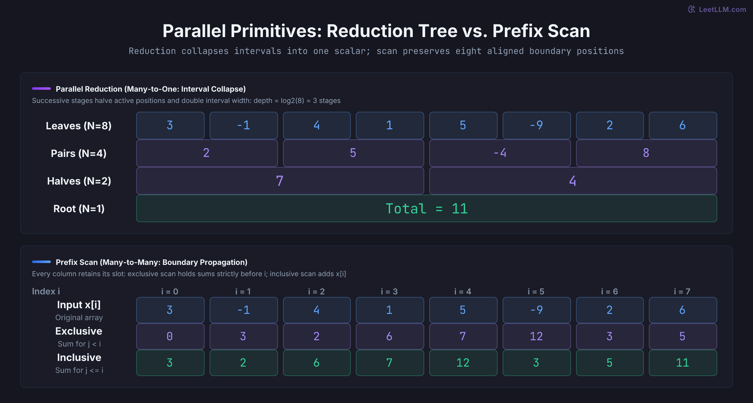
Pair adjacent values in the running array [3, -1, 4, 1, 5, -9, 2, 6]. Adding neighboring pairs at the first level yields [2, 5, -4, 8]. Combining those adjacent sums at the second level yields [7, 4]. The final addition produces 11. A balanced reduction tree with $n$ leaves requires $n-1$ additions and $\log_2 n$ sequential combining steps.

A prefix scan asks for a completely different contract: it keeps every intermediate boundary. An exclusive sum at index $i$ accumulates elements strictly before index $i$, placing the additive identity 0 at index 0. An inclusive sum also includes $x_i$. For the first four elements [3, -1, 4, 1], the exclusive prefix sum is [0, 3, 2, 6] and the inclusive prefix sum is [3, 2, 6, 7].

For exact real addition, the two scan conventions connect through a direct identity:

$$\operatorname{inclusive}[i]=\operatorname{exclusive}[i]+x_i.$$

Arg reduction carries a structured payload: (value=6, index=7). When multiple positions share the maximum, you must pair the comparison operator with a deterministic tie-breaking rule, such as picking the lowest index. The Python reference below verifies all three primitive contracts before introducing GPU hardware details.

Reduce within a warp using shuffle intrinsics

Early GPU reduction kernels relied heavily on shared memory: threads wrote inputs into a __shared__ array, synchronized via __syncthreads(), and accumulated across stride intervals. That approach cost shared memory capacity, suffered from bank conflicts when strided accesses hit identical memory banks, and stalled on block barriers at every tree level.

Modern CUDA warps (32 threads) bypass shared memory completely by using warp shuffle intrinsics like __shfl_down_sync. Shuffle instructions let threads read register values directly from other lanes within the same warp across the streaming multiprocessor's crossbar, delivering single-cycle register-to-register communication.^{[1]Reference 1C/C++ Language Extensionshttps://docs.nvidia.com/cuda/cuda-programming-guide/05-appendices/cpp-language-extensions.html}

Offsets 16, 8, 4, 2, 1 construct a five-stage reduction tree across all 32 lanes. Lane 0 accumulates the warp total, while higher lanes hold intermediate partials:

Two hardware rules govern this kernel. First, starting with the Volta architecture, NVIDIA GPUs run with Independent Thread Scheduling. Before Volta, all 32 threads in a warp shared a single program counter and executed in lockstep. On modern architectures, threads maintain independent program counters and call stacks. Omitting a mask or relying on implicit lockstep execution leads to divergence bugs. The active mask kFullMask = 0xffffffffu explicitly forces all 32 lanes to synchronize at each shuffle step.^{[2]Reference 2CUDA Programming Guide.https://docs.nvidia.com/cuda/cuda-programming-guide/}

Second, participating in the shuffle is separate from adding the result. If a warp processes only 20 active inputs, threads 20 through 31 shouldn't exit early. In CUDA's shuffle contract, reading from an exited or non-participating lane returns an undefined value or the caller's own value. If lane 4 reads from lane $4+16=20$ and lane 20 has exited, lane 4 receives its own value and doubles it. Feeding 0 into inactive lanes and running the full mask guarantees that every source lane contributes the additive identity. The conditional addition if (lane + offset < warpSize) belongs strictly after the shuffle instruction so that all lanes execute the collective together.

The CPU model verifies this behavior by checking lane participation, missing source rejections, and signed 64-bit integer overflow protection:

To aggregate across a 256-thread block (8 warps), lane 0 of each warp deposits its warp total into __shared__ long long warp_sums[8]. A block-wide barrier __syncthreads() guarantees all 8 warps finish their writes before warp 0 reads the shared array. Warp 0's first 8 lanes load the 8 partial sums, while lanes 8 through 31 load zero. A second warp_sum folds those 8 partials, leaving the entire block total in lane 0:

Notice the barrier placement: __syncthreads() sits outside all warp-divergent branches. Placing a block barrier inside if (lane == 0) or if (warp == 0) triggers undefined behavior because only a fraction of the block's threads reach the barrier.

Aggregate partials across blocks: multi-pass kernels versus global atomics

Each thread in the block loads two elements: one at block_start + threadIdx.x and one 256 elements later. Consecutive threads access consecutive memory addresses, ensuring fully coalesced global memory loads.^{[3]Reference 3Optimizing Parallel Reduction in CUDAhttps://developer.download.nvidia.com/compute/cuda/1.1-Beta/x86_website/projects/reduction/doc/reduction.pdf} A 256-thread block consumes 512 input elements and emits a single 64-bit block partial.

To reduce across thousands of blocks, why can't we just synchronize the entire grid inside one kernel? Because GPUs don't provide a general grid-wide barrier across independent thread blocks. Blocks execute dynamically across available Streaming Multiprocessors. If a kernel paused waiting for unlaunched blocks that can't fit on the SMs due to occupancy limits, the GPU would deadlock.

Two architectural strategies solve this grid-scale aggregation:

1. Multi-pass hierarchical kernel launches: Each kernel pass reduces elements by a factor of 512. For 4,194,304 inputs:

Because the host queues all three launches in the same CUDA stream, the hardware guarantees they execute sequentially without race conditions. Each pass streams data in wide, coalesced bursts across all memory channels, avoiding write contention.

1. Global atomics (atomicAdd): In this approach, each block reduces its local tile and uses atomicAdd(&global_sum, block_sum) to update a single output location in global memory.

• When atomics make sense: If the grid has few blocks, or if you're reducing into many independent output bins (like histogramming or channel-wise normalization), atomic contention is minimal.
• When atomics crawl: When thousands of blocks all finish nearly simultaneously and attempt an atomicAdd on the exact same 64-bit address, the memory controllers in the L2 cache slice serialize all requests. The pipeline stalls waiting for read-modify-write transactions to queue up.

The hierarchical multi-pass approach eliminates serialization entirely, trading small launch overhead for clean bandwidth scaling.

Floating-point trees can disagree without a race

Integer addition is associative and commutative, so grouping and ordering don't alter the mathematical result (provided no intermediate overflows). Real numbers are also associative, but IEEE 754 floating-point addition rounds after every single operation. Floating-point addition is commutative ($a + b = b + a$), but it's not associative:

$$(a + b) + c \neq a + (b + c).$$

The standard library example below forces 32-bit float truncation to reveal how operand ordering changes low bits on identical inputs:

In a parallel GPU reduction, thread block execution order is nondeterministic across SMs. If blocks complete in different orders, or if a dynamic schedule alters which block partials combine first, the low-order mantissa bits vary between runs.

This bitwise difference doesn't mean there's a race condition or a bug. It's the natural consequence of floating-point non-associativity across dynamic parallel trees.

Repeatability and numerical accuracy are two distinct properties:

• Repeatability (determinism) guarantees that running the kernel twice on the same input produces the exact same bit pattern. CUB's DeviceReduce provides run_to_run determinism by fixing the internal tile reduction order.^{[4]Reference 4cub::DeviceReducehttps://nvidia.github.io/cccl/unstable/cub/api/structcub_1_1DeviceReduce.html} But bitwise repeatability doesn't prove the result is close to the true mathematical sum.
• Accuracy measures how close the computed float is to infinite-precision arithmetic. A balanced pairwise summation tree is generally far more accurate than serial accumulation because it avoids adding tiny numbers to massive running totals, even if scheduling differences cause tiny bit variations across runs. When verifying float kernels, always compare against a higher-precision reference using explicit relative and absolute tolerances rather than testing for bitwise equality.

Parallel scan: Hillis-Steele step efficiency versus Blelloch work efficiency

While reduction collapses an array into one value, prefix scan distributes cumulative prefixes back to every element. Two classic parallel algorithms tackle prefix scan with different complexity trade-offs:

• Hillis-Steele (Step-efficient): In each step $k$ (with stride $2^k$), every active thread $i$ adds the element at $i - 2^k$. It completes in only $\log_2 n$ steps. However, every step performs additions across almost the entire array, yielding $O(n \log n)$ total work. Hillis-Steele is ideal inside a single 32-lane warp via __shfl_up_sync: because all 32 lanes execute in parallel on the warp's ALUs in 5 steps, the extra additions don't waste instruction cycles because inactive lanes are merely masked out.

• Blelloch (Work-efficient): Blelloch scan takes $2 \log_2 n$ steps, but performs only $O(n)$ additions ($2n - 2$ operations total). It splits the scan into two distinct phases in shared memory:

1. Up-Sweep (Reduce): A binary reduction tree where stride doubles each round (1, 2, 4, ...). Threads add values upward until the root (last array position) holds the grand total.
2. Down-Sweep (Distribute): Save the root total, overwrite the root with 0 (the additive identity), and reverse the tree with stride halving (... 4, 2, 1). At each step, a node sends its current value to its left child, while its right child receives the sum of its old left child and its current value.

For a 512-item block, Hillis-Steele requires roughly $512 \times 9 \approx 4,608$ additions, whereas Blelloch needs only $2 \times 512 - 2 = 1,022$ additions: a $4.5\times$ reduction in shared-memory traffic and arithmetic operations.^{[5]Reference 5Single-pass Parallel Prefix Scan with Decoupled Look-backhttps://research.nvidia.com/sites/default/files/pubs/2016-03_Single-pass-Parallel-Prefix/nvr-2016-002.pdf}

The trace below captures the exact array mutations during Blelloch exclusive scan on [3, -1, 4, 1]:

Propagate block offsets: multi-pass hierarchies versus decoupled look-back

A local Blelloch scan computes correct prefixes within each block, but every block starts at local offset 0. To stitch them into a device-wide prefix scan, each block must receive the cumulative sum of all preceding blocks.

In a hierarchical multi-pass scan:

1. Each block scans its 512 elements, emits local prefixes, and writes its block total to a global block_sums buffer. For blocks with inputs [3,-1,4,1] and [5,-9,2,6], the block totals are [7, 4].
2. A second kernel scans block_sums to compute block offsets: exclusive_scan([7, 4]) = [0, 7].
3. A third kernel broadcasts each block's offset across its threads: Block 0 adds +0, while Block 1 adds +7 to all its local prefixes, converting [0, 5, -4, -2] into [7, 12, 3, 5].

Testing scan hierarchies requires exercising recursion boundaries. If your block size is 512, an input of $512^2 = 262,144$ elements produces exactly 512 block totals, which fit in a single metadata block. But $512^2 + 1 = 262,145$ elements produce 513 block totals, spilling into two metadata blocks and triggering another recursion level. Testing only small powers of two misses that structural threshold.

Decoupled Look-Back (Single-Pass Scan): Multi-pass scan requires three kernel launches and writes all intermediate block totals to global memory. NVIDIA CUB's DeviceScan eliminates intermediate launches using decoupled look-back (Merrill & Garland 2016):^{[5]Reference 5Single-pass Parallel Prefix Scan with Decoupled Look-backhttps://research.nvidia.com/sites/default/files/pubs/2016-03_Single-pass-Parallel-Prefix/nvr-2016-002.pdf}

• Blocks grab dynamic tile indices via an atomic counter.
• Each block computes its local reduction aggregate and publishes a status flag in global memory:
  • X: Uninitialized.
  • A: Local aggregate computed and published.
  • P: Inclusive prefix across all prior tiles computed and published.
• When block $k$ finishes its local aggregate, it looks back at tile $k-1$:
  • If tile $k-1$ is marked P, block $k$ reads the prefix directly, adds its local aggregate, and publishes its own status P.
  • If tile $k-1$ is marked A, block $k$ adds tile $k-1$'s aggregate and looks further back to tile $k-2$, accumulating aggregates until it reaches a tile marked P.

Decoupled look-back achieves a single-pass device scan with approximately $n$ global memory reads and $n$ global memory writes, overlapping prefix propagation directly with tile computation.^{[6]Reference 6cub::DeviceScanhttps://nvidia.github.io/cccl/unstable/cub/api/structcub_1_1DeviceScan.html}

Online softmax carries a scale with its sum

Softmax converts an array of unnormalized logits $x_i$ into a probability distribution:

$$p_i = \frac{e^{x_i - m}}{\sum_j e^{x_j - m}}, \qquad m = \max_j x_j.$$

Subtracting the maximum $m$ prevents floating-point overflow when evaluating exponentials.

A conventional 3-pass GPU softmax makes three full trips across global memory (HBM):

1. Reduction pass: find the global maximum $m = \max_j x_j$.
2. Reduction pass: compute the normalizer denominator $d = \sum_j e^{x_j - m}$.
3. Elementwise pass: compute each probability $p_i = e^{x_i - m} / d$.

When tensors are large, those three memory round trips throttle performance on memory-bandwidth-bound GPUs.

The online normalizer (Milakov & Gimelshein 2018) merges the maximum search and exponential summation into a single pass.^{[7]Reference 7Online normalizer calculation for softmax.https://arxiv.org/abs/1805.02867} It maintains a running state tuple $(m, d)$, where $m$ is the running maximum and $d$ is the exponential sum measured relative to that maximum.

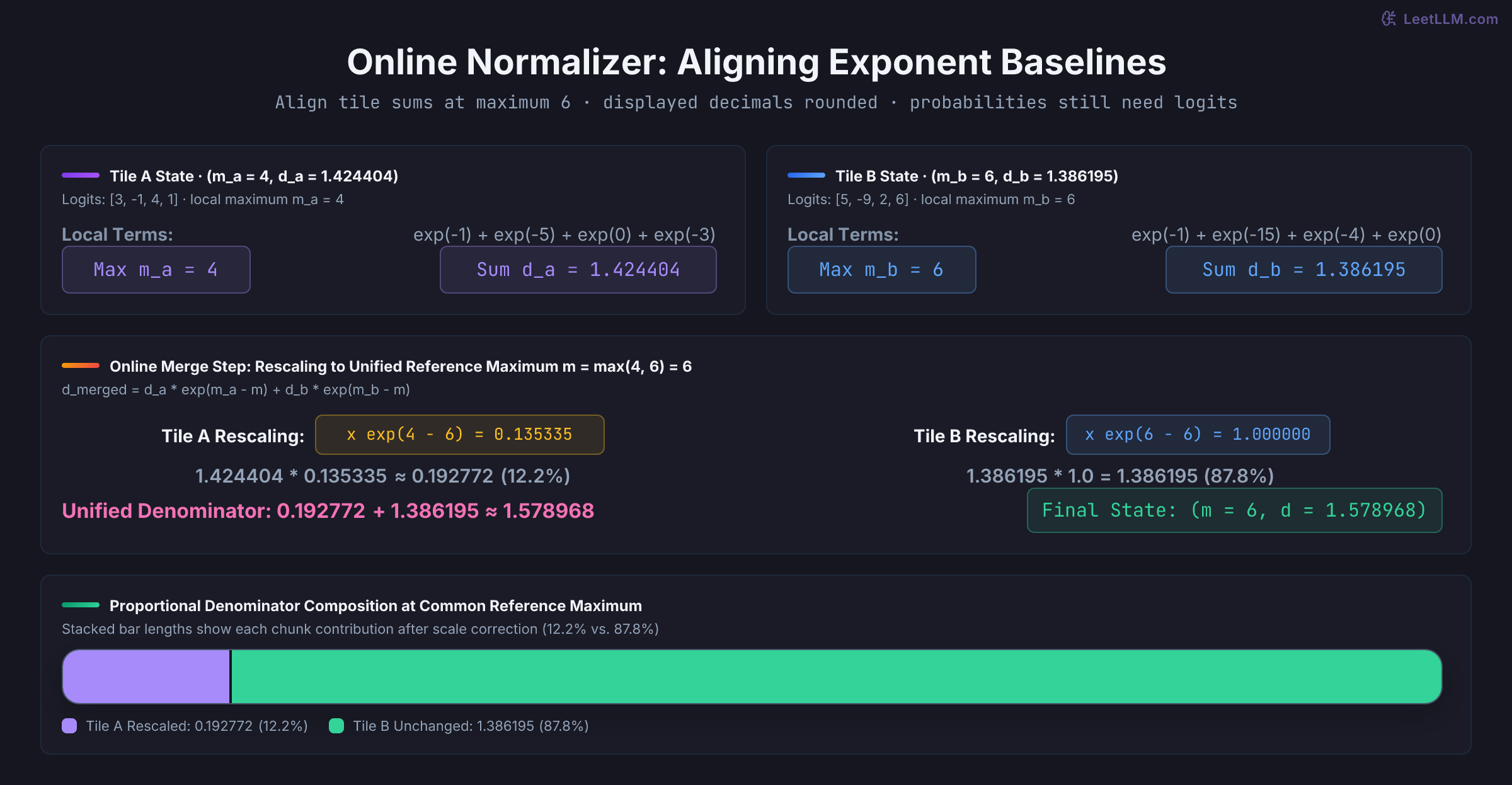
When merging two partial states $(m_a, d_a)$ and $(m_b, d_b)$, the combined maximum is $m = \max(m_a, m_b)$. Before adding the sums, each denominator must be rescaled to match the new reference point:

$$m = \max(m_a, m_b), \qquad d = d_a e^{m_a - m} + d_b e^{m_b - m}.$$

For our running array partitioned into two halves, $x_{\text{left}} = [3, -1, 4, 1]$ has $m_a = 4$ and $d_a \approx 1.424404$. The right half $x_{\text{right}} = [5, -9, 2, 6]$ has $m_b = 6$ and $d_b \approx 1.386195$. When merging, the global maximum becomes 6. The left denominator shrinks by $e^{4 - 6} = e^{-2} \approx 0.135335$ to become $0.192772$, while the right denominator stays unchanged. Adding them gives the exact combined denominator $1.578968$.

How FlashAttention builds on the online normalizer: This online state update is the foundation behind FlashAttention (Dao et al., 2022).^{[8]Reference 8FlashAttention: Fast and Memory-Efficient Exact Attention with IO-Awareness.https://arxiv.org/abs/2205.14135} Standard attention computes $S = QK^T$, takes the full softmax $P = \operatorname{softmax}(S)$, and multiplies by $V$, materializing an $N \times N$ attention matrix in HBM ($O(N^2)$ memory traffic).

FlashAttention loads blocks of $Q$, $K$, and $V$ into fast SRAM (shared memory/registers). For each block of keys and values, it computes local dot products $S_{\text{tile}}$, updates the running online softmax state $(m, d)$, and rescales the accumulated output accumulator $O$ in registers:

$$O_{\text{new}} = \operatorname{diag}\left(e^{m_{\text{old}} - m_{\text{new}}}\right) O_{\text{old}} + e^{S_{\text{tile}} - m_{\text{new}}} V_{\text{tile}}.$$

At the end of the sequence, it divides $O$ by the final accumulated denominator $d$. The $N \times N$ attention probabilities are never written to HBM, shrinking memory footprint from $O(N^2)$ to $O(N)$ and turning bandwidth-choked attention into compute-bound tensor core math.

Race conditions and verification: sanitizing shared-memory hazards

Parallel primitives push shared memory to its limit. Threads within a block constantly exchange data through shared arrays. Writing correct parallel primitives requires catching three subtle classes of data hazards:

• RAW (Read-After-Write): Thread A writes to a shared index, but Thread B reads before the write finishes.
• WAR (Write-After-Read): Thread A reads from a shared location, but Thread B overwrites that location before Thread A finishes loading.
• WAW (Write-After-Write): Multiple threads attempt to write to the same shared address without a deterministic sequence.

NVIDIA's Compute Sanitizer provides specialized tools to detect these defects at the machine-instruction level:^{[9]Reference 9Compute Sanitizerhttps://docs.nvidia.com/compute-sanitizer/ComputeSanitizer/}

Each tool addresses a specific failure mode:

1. synccheck validates barrier usage. If threads within a block call __syncthreads() inside divergent branches (where some threads participate while others take an alternative path), the hardware can deadlock or hang. synccheck verifies that all non-exited threads in a block reach the identical barrier instruction.
2. racecheck tracks shared memory accesses dynamically. It records the cycle and warp of every load and store. If two threads access the same shared memory location without an intervening __syncthreads() or __syncwarp(), racecheck flags the exact instruction and line number.
3. memcheck detects out-of-bounds reads and writes in global and shared memory, plus unaligned memory accesses.

Keep two verification rules firmly separated:

• A clean sanitizer run doesn't prove arithmetic correctness. If your scan kernel forgets to add block offsets, racecheck reports 0 hazards because there are no race conditions, but every output value in block 1 will be wrong.
• A passing test run doesn't prove race-freedom. On an idle GPU running a small test, warps might serendipitously execute in order and produce the correct output. But under production load with multiple kernels competing for SM resources, that hidden race condition will corrupt output buffers. Always run both reference assertions and Compute Sanitizer tools.

Select the primitive by its output contract

Different workloads demand different output contracts:

For standalone collective operations on whole arrays, prefer NVIDIA CUB (cub::DeviceReduce, cub::DeviceScan, cub::BlockScan).^{[10]Reference 10CUB Developer Overviewhttps://nvidia.github.io/cccl/unstable/cub/developer_overview.html} CUB is part of NVIDIA's CUDA Core Compute Libraries (CCCL). It features tuned architecture-specific policies, auto-tuning for different GPU generations, and optimized decoupled look-back implementations.

CUB's device-wide APIs use a two-step allocation pattern: query the required scratchpad size with a nullptr, allocate memory, then execute:

When should you write a custom collective kernel instead of calling CUB?

1. Kernel fusion: If reduction or scan is only one step of a larger workflow (such as online softmax inside attention, LayerNorm, or RoPE), calling CUB forces you to write intermediate tensors to HBM and launch separate kernels. Fusing the primitive directly inside your custom kernel keeps data in registers and shared memory.
2. Specialized tensor layouts: If your data resides in register-tiled GEMM fragments or strided multi-dimensional buffers that CUB's linear iterators can't map, custom warp and block primitives are essential.

Run the CUDA lab and verify correctness boundaries

Download the CUDA source code into your working environment:

• The CUDA lab source
• Host validation header
• CPU algorithm model
• Historical benchmark receipt

Compile with full optimization and line information:

Before benchmarking, run correctness sweeps across warp boundaries (31, 32, 33), block boundaries (255, 256, 257, 511, 512, 513), and recursive scan boundaries ($512^2 + 1 = 262,145$):

CPU checks you can run immediately

The companion Python model verifies these same index boundaries, checking 17 hierarchy sizes, 260 recursive scan cases, signed overflow handling, and online softmax partition merges:

Interpret timing without confusing traffic and bandwidth

The benchmark measures elapsed time using CUDA events across 30 iterations after 5 warmup cycles. Allocation and initial host-to-device transfers are excluded from timing.

The benchmark reports logical byte rate:

• For reduction: $4N$ input bytes divided by elapsed time.
• For scan: $4N$ input bytes plus $8N$ output bytes ($12N$ bytes total) divided by elapsed time.

This logical rate reflects algorithmic data volume, not physical DRAM transactions. It doesn't include intermediate scratchpad writes or cache hits in L2. Always record compiler flags, CUDA toolkit versions, GPU architecture, and profiler metrics (such as memory throughput from NCU) when reporting performance numbers.

Review questions

1. Why does warp shuffle avoid shared memory bank conflicts during intra-warp reduction?

Shuffle intrinsics exchange register contents directly over hardware crossbar interconnects within the 32-lane warp. They require zero shared memory allocation, generate no memory transactions, and eliminate block-wide __syncthreads() barriers.

2. What is the fundamental algorithmic tradeoff between Hillis-Steele and Blelloch parallel scan?

Hillis-Steele executes $\log_2 N$ steps with $O(N \log_2 N)$ total additions, prioritizing step efficiency at the expense of work efficiency. Blelloch splits execution into Up-Sweep reduction and Down-Sweep distribution phases taking $2 \log_2 N$ steps but only $O(N)$ operations, matching serial work complexity.

3. Why do floating-point parallel reductions yield non-identical results across different tile configurations?

IEEE 754 floating-point addition is non-associative: $(a + b) + c \neq a + (b + c)$. Altering thread block dimensions, tile sizes, or reduction tree hierarchies shifts intermediate rounding boundaries, producing slight bitwise discrepancies even in strictly race-free code.

4. How does decoupled look-back eliminate multi-pass kernel launches in global prefix scans?

In decoupled look-back, blocks publish their local status and running totals into global state flags using release consistency. Downstream blocks inspect upstream flags directly, either consuming completed prefixes or accumulating partial aggregates dynamically without terminating the kernel grid.

5. Why does online softmax rescale running accumulators when updating the maximum?

Online softmax applies the algebraic identity $e^{x - m_{\text{new}}} = e^{x - m_{\text{old}}} \cdot e^{m_{\text{old}} - m_{\text{new}}}$. When encountering an element larger than the current maximum, the kernel rescales its existing exponential sum in registers by $e^{m_{\text{old}} - m_{\text{new}}}$, maintaining numerical stability in a single pass without intermediate HBM writes.