Bayesian Inference from Evidence

A coding agent passes eight of ten held-out tasks. Is its success rate above 70%? The observed rate is 80%, but ten tasks leave room for luck. We need to distinguish a promising estimate from strong evidence that the agent clears the threshold.

Probability for Machine Learning introduced base rates and conditioning. Bayesian inference applies the same reasoning to an unknown model parameter: state which values were plausible before the evaluation, then update those beliefs using the results. The answer is a distribution of plausible success rates, not just one adjusted score.^{[1]Reference 1Machine Learning: A Probabilistic Perspective.https://probml.github.io/pml-book/book0.html}

We'll use those same eight passes and two failures throughout. Start with a mild preference for middle success rates, then change that preference to see how much the conclusion depends on it.

Formulating the unknown success parameter

Let $p$ mean the probability that this agent passes a randomly drawn task from the intended deployment population. Pin the agent's model, prompt, tools, retry budget, and pass criterion. One observation is one task evaluated under that fixed policy.

Our simple model treats the outcomes as independent conditional on $p$, with the same success probability for each draw. That means: if we knew $p$, knowing one result wouldn't change the probability of another. Tasks can differ in difficulty, but their sampling process must stay the same. Ten handpicked easy tasks won't support a claim about a different production mix.

The direction of conditioning matters. A likelihood asks about the data given a proposed rate. A posterior asks about the rate given the data. Bayes' rule connects them; they aren't interchangeable.

Binomial likelihood scores candidate success rates

At a candidate rate of 0.8, each pass contributes a factor of 0.8 and each failure contributes 0.2. One particular sequence of eight passes and two failures has probability $0.8^8 \times 0.2^2$. There are 45 possible positions for the two failures, so the probability of exactly eight passes, regardless of order, is 45 times that value.

Python's comb(10, 8) counts the 45 unique arrangements of eight passes across ten trials. Evaluating this binomial formula across candidate rates reveals how sharply the observed run separates hypotheses:

The eight-pass result is about 6.9 times as likely at rate 0.8 as at rate 0.5. That favors 0.8 relative to 0.5, but it doesn't mean there's a 30.2% posterior probability that the rate is 0.8. We haven't combined the evidence with a prior.

For a general candidate rate, the likelihood is $45p^8(1-p)^2$. The factor 45 is the same for every candidate, so it cancels when we normalize the posterior. We can therefore work with a likelihood proportional to $p^8(1-p)^2$. The symbol $\propto$ means "equal up to a constant factor."

Beta distributions quantify prior beliefs

A beta distribution describes uncertainty about a probability between 0 and 1. Its two positive shape parameters, $\alpha$ and $\beta$, control where that uncertainty sits. We'll choose Beta(2, 2): it favors middle rates over near-zero or near-one rates, without ruling out a broad range.

This is an explicit modeling choice, not a claim that we observed two historical passes and two failures. A uniform Beta(1, 1) prior would give equal density to all rates. Increasing both parameters equally concentrates the distribution around 0.5. These alternatives make it possible to test how much the prior matters.

For a continuous rate, probability belongs to a range of values, represented by area under a density curve. The height at one point isn't a probability and can exceed 1. Beta(2, 2) has density $6p(1-p)$; the constant 6 makes the total area from 0 to 1 equal to 1.^{[2]Reference 2scipy.stats.betahttps://docs.scipy.org/doc/scipy/reference/generated/scipy.stats.beta.html}

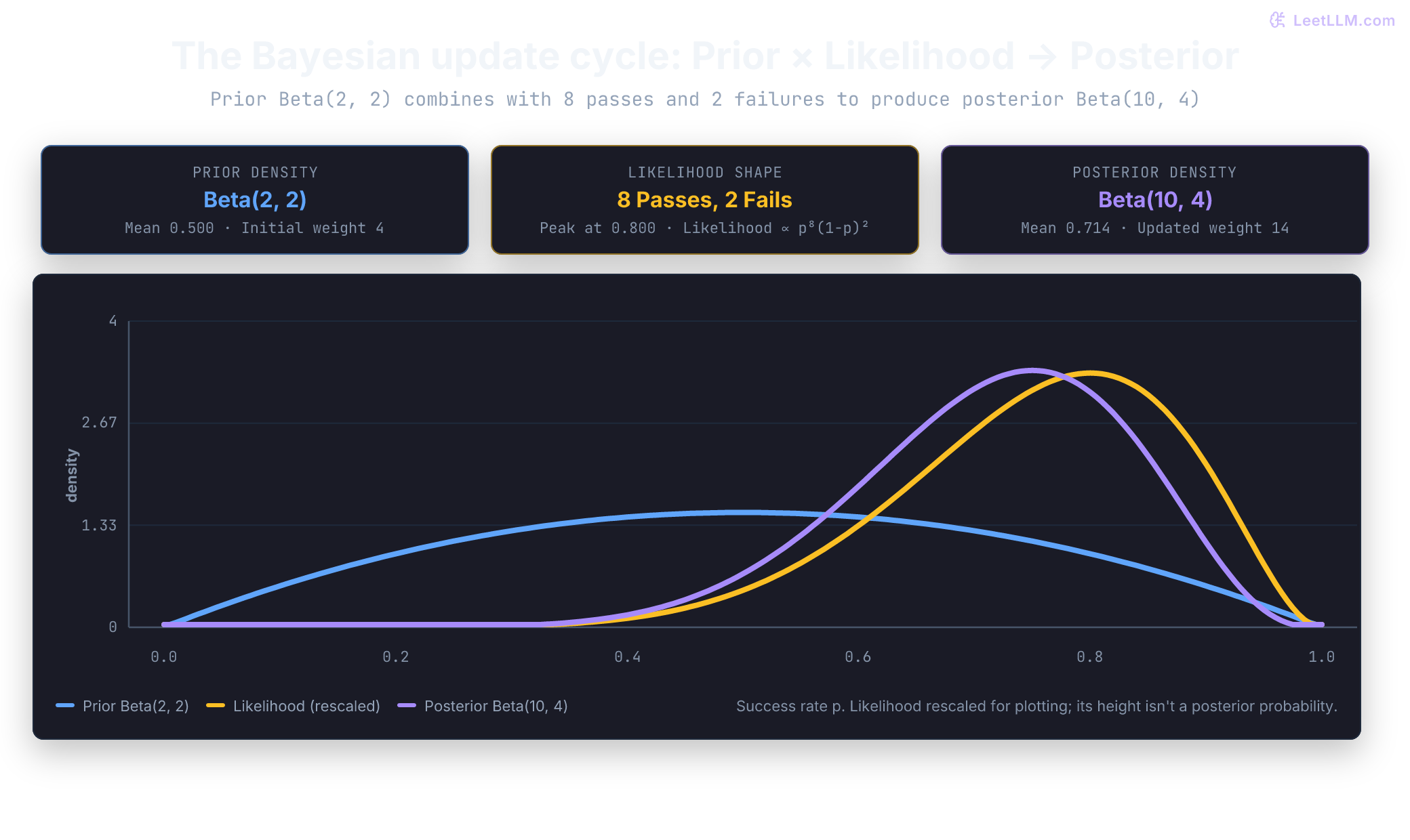
Bayes' rule multiplies that prior shape by the likelihood, then rescales the result so its total area is 1:

$$\text{posterior density} \propto \text{prior density} \times \text{likelihood}$$

For our run, multiplying $p(1-p)$ by $p^8(1-p)^2$ gives $p^9(1-p)^3$. A beta density has the shape $p^{\alpha-1}(1-p)^{\beta-1}$, so the new exponents identify Beta(10, 4). The prior's exponents and the data's exponents add; the observations don't replace the prior.^{[3]Reference 3Gittins Index for Bayesian Bandits: Beta-Binomial Conjugacyhttps://www.stat.berkeley.edu/~bartlett/courses/2014fall-cs294stat260/lectures/gittins-notes.pdf}

Beta-binomial conjugacy produces an exact posterior

Now the arithmetic has a reason behind it: $2+8=10$ and $2+2=4$. A beta prior combined with a binomial count likelihood stays in the beta family. This makes beta a conjugate prior for that likelihood. For any observed data $D$ containing $s$ passes and $f$ failures:

$$p \mid D \sim \operatorname{Beta}(\alpha+s,\;\beta+f)$$

Here $\alpha$ and $\beta$ are the prior parameters, $s$ counts observed passes, and $f$ counts observed failures. Substitute the actual numbers:

$$\operatorname{Beta}(2+8,\;2+2)=\operatorname{Beta}(10,4)$$

Posterior expectation is given by:

$$E[p\mid D]=\frac{\alpha+s}{\alpha+\beta+s+f}=\frac{10}{14}\approx0.714$$

Observed alone, the empirical pass fraction is $8/10=0.800$. Before seeing any runs, the prior mean was $2/4=0.500$. After the update, the posterior mean resolves to an exact weighted average of those two quantities:

$$\frac{4}{14}\times0.5 + \frac{10}{14}\times0.8 = \frac{10}{14}$$

Here the prior holds weight 4 while the empirical runs contribute weight 10. These weights explain the gravitational pull toward 0.5; they don't mean anyone actually ran four historical benchmark tasks.

The next cell repeats that arithmetic and checks the parameter totals before printing the updated rate.

Forecasting the next run with the posterior predictive

If the next task is comparable, the posterior predictive probability gives a forecast before it runs. To forecast the outcome of the eleventh task, average each candidate success rate weighted by its posterior credibility. At rate 0.6, the next task has pass probability 0.6; at rate 0.8, it has probability 0.8. Integrating over the entire Beta(10, 4) distribution yields an expected future pass probability equal to the posterior mean, $10/14\approx0.714$.^{[3]Reference 3Gittins Index for Bayesian Bandits: Beta-Binomial Conjugacyhttps://www.stat.berkeley.edu/~bartlett/courses/2014fall-cs294stat260/lectures/gittins-notes.pdf}

This reflects uncertainty about a future outcome, not a claim that $p$ is exactly 0.714. If the next task passes, the posterior becomes Beta(11, 4), and the following task's forecast rises to $11/15\approx0.733$. Sequential updates and one combined update give the same parameters when they use the same observations and model.

Why does the posterior mean equal 10/14 instead of the observed pass rate 8/10?

Answer

The Beta(2,2) prior contributes parameter weights of 2 and 2. Combining them with eight passes and two failures yields Beta(10,4), whose mean is 10 divided by 14. Those prior weights are assumptions, not extra observed tasks.

Prior sensitivity: when assumptions outweigh small samples

Two engineers can see the same ten outcomes and reach different posterior means because they chose different priors. Hold the observations fixed and vary only the starting assumption.

The next cell reuses the pass and failure counts and compares a weak Beta(1, 1) prior, a moderate Beta(2, 2) prior, and a strong Beta(20, 20) prior. Predict what should happen before reading the numbers: the strong prior should stay closer to 0.5.

Beta(20, 20) gives its starting mean a weight of 40, compared with 10 for the new data. The updated mean is therefore $0.8\times0.5+0.2\times0.8=0.56$. That strength needs justification, such as substantial evidence that genuinely applies to this agent and task population.

Relative to a uniform Beta(1, 1) baseline, reaching Beta(20, 20) would require 19 historical passes and 19 historical failures, not 40 observed tasks. Parameter weights function as bookkeeping; they aren't provenance records. Keep those two facts separate.

Report several defensible priors when the sample is small. If the deployment decision flips between them, collect more representative evidence instead of quietly choosing the prior that makes the preferred outcome win.

An engineer claims Beta(20,20) proves that 40 comparable historical tasks were observed. What information is missing?

Answer

The prior has total parameter weight 40, but that weight isn't automatically 40 observed tasks. Relative to a uniform Beta(1,1) baseline, the same prior could result from 19 historical passes and 19 historical failures. The earlier baseline and the historical evidence's provenance must both be disclosed.

Credible intervals and tail probabilities versus point averages

A mean of 0.714 leaves our original question unanswered: how much evidence says the rate exceeds 0.7? Beta(10, 4) assigns probability both below and above that threshold.

A 90% equal-tailed credible interval leaves 5% of the posterior area below its lower endpoint and 5% above its upper endpoint. The remaining 90% lies between them. These endpoints are the 5th and 95th quantiles, or percentile cutoffs, of the posterior.

SciPy's beta.ppf returns those cutoffs. Its beta.sf(0.7, a, b) returns the area above 0.7, which directly answers our threshold question.^{[2]Reference 2scipy.stats.betahttps://docs.scipy.org/doc/scipy/reference/generated/scipy.stats.beta.html} Use the same Beta(10, 4) posterior for both calculations:

Calculating the quantiles yields an interval of [0.505, 0.887], while the posterior probability above 0.7 is only 0.579. Having an expected value of 0.714 doesn't mean you're confident the agent clears 0.70; in fact, there's a 42.1% chance its true rate falls below your release bar!

Crucially, this interval reflects parameter uncertainty under the chosen prior and binomial model. Tasks themselves don't yield fractional outputs: each run either succeeds or fails. Frequentist procedures interpret intervals differently, evaluating long-run coverage under repeated sampling. Subsequent lessons explore those distinctions in detail.

Another summary is the posterior standard deviation, which measures spread around the mean. Its square, the variance, has a closed form for Beta($a,b$):

$$\operatorname{Var}(p\mid D)=\frac{ab}{(a+b)^2(a+b+1)}$$

At Beta(10, 4), the variance is $40/(196\cdot15)\approx0.0136$, and its square root is about 0.117. Use beta quantiles for the interval above; a shortcut such as mean plus or minus two standard deviations needn't give the intended probability, especially near 0 or 1.

The posterior mean exceeds 0.7. Does the posterior assign at least 90% probability to rates above 0.7?

Answer

No. The mean is 0.714, but the posterior area above 0.7 is only about 0.579. The average and the probability of clearing a threshold answer different questions.

Sample size scaling: comparing 8/10 against 80/100

Hold the Beta(2, 2) prior fixed and compare two alternative sample sizes: eight passes out of ten and eighty passes out of one hundred. Both observed rates are 0.8. The larger run yields Beta(82, 22), not Beta(90, 24): we're replacing the ten-task example with a hundred-task example, not adding the runs together.

The next independent cell computes both means, standard deviations, and equal-tailed intervals. Predict which interval will be narrower before running it:

With one hundred tasks, the posterior mean moves to 0.788, the spread tightens dramatically, and the 90% credible interval contracts to [0.720, 0.851]. Posterior tail probability above 0.7 jumps from 57.9% to 98.1%. That contrast shows why sample size transforms raw fractions into actionable decisions: identical 80% empirical rates deliver completely opposite degrees of certainty.

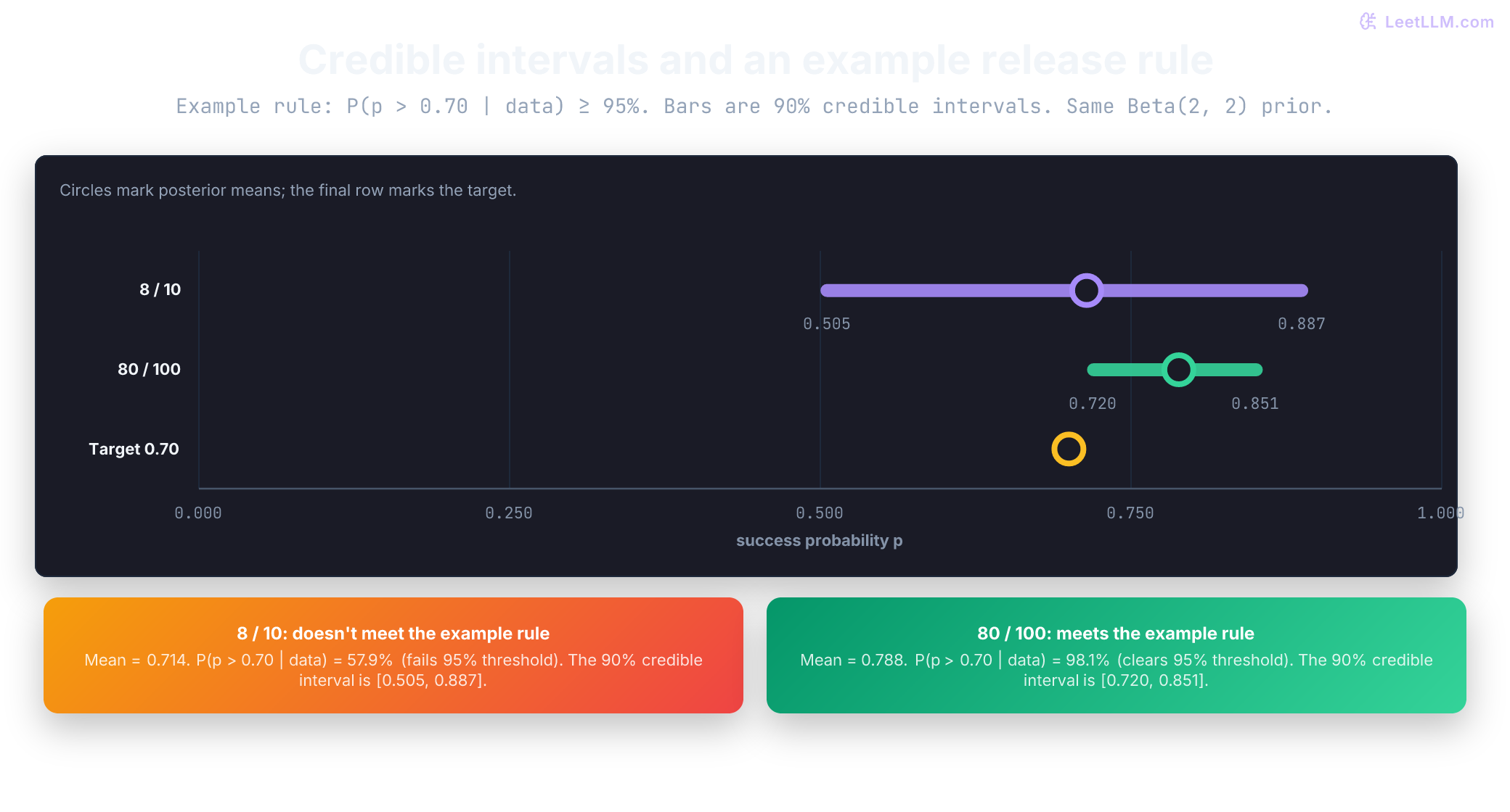
More data doesn't remove randomness from individual future tasks. Even if we learned that $p$ was exactly 0.8, a new task could still fail. It also doesn't remove uncertainty caused by a wrong model or an unrepresentative sample.

Posterior dispersion versus empirical calibration

Posterior spread and calibration answer different questions. The posterior describes uncertainty about a success rate under a chosen model. Calibration asks whether forecasts line up with later outcomes: among many comparable tasks assigned a pass probability near 0.7, do about 70% pass?

A frozen 0.714 forecast can't establish calibration from the same ten tasks that produced it. Save forecasts before later outcomes arrive. Across enough predictions, group similar probabilities and compare each group's average forecast with its observed pass fraction.^{[4]Reference 4On Calibration of Modern Neural Networkshttps://arxiv.org/abs/1706.04599} With only one frozen forecast, this amounts to comparing that forecast with the pass fraction on a fresh batch.

Small batches fluctuate, so one mismatch isn't proof of a bad model. Persistent discrepancies deserve investigation: did the task mix shift, were retries counted as new tasks, or did the agent's policy change? More data can narrow a wrong model's posterior without making its predictions reliable.

Sampling failure modes that corrupt the posterior

The arithmetic can be correct while the inference is wrong.

Keep the collection and reporting process visible. Omitted runs, selected agents, or an undisclosed change of target population can make the reported analysis answer a different question from the one a reader assumes. Updating can't turn duplicated or biased rows into representative observations.

A model passes eight out of ten tasks, but all ten rows are retries of the same prompt. Why is Beta(10,4) misleading?

Answer

The intended parameter describes new tasks from the deployment population. Ten retries of one prompt mainly describe that prompt. Even if retry randomness is independent, the prompt wasn't sampled ten times independently from that population. A beta update might model that prompt's retry success rate, but it doesn't establish the broader task success rate.

Production release gates with posterior decision rules

For this exercise, choose the rule before seeing results: increase traffic only if the posterior probability that $p>0.7$ is at least 95%. This is an illustrative evidence threshold, not a universal release policy. Real decisions also depend on the cost of failures, traffic exposure, and other safety checks.

Under Beta(2, 2), the ten-task result doesn't pass this rule: 0.579 < 0.95. The hundred-task result does: 0.981 > 0.95, provided its tasks and policy satisfy the model assumptions. Neither decision follows from the raw 80% rate alone.

Try these changes before reading the answers:

1. One more comparable task fails after the original eight passes and two failures. What are the new posterior and next-task forecast?
2. Apply the 95% evidence rule to the original ten outcomes with Beta(1, 1) and Beta(20, 20) priors. Use beta.sf(0.7, a, b), not just the mean. Does either pass?
3. Could the hundred-task result justify the same claim if every task came from an unusually easy benchmark family?

Decision and sensitivity analysis checks

1. Add the failure once: Beta(10, 5), with forecast $10/15\approx0.667$. Don't add the original ten observations again when starting from their posterior.
2. Posteriors update to Beta(9, 3) and Beta(28, 22). Their probabilities above 0.7 evaluate to 0.687 and 0.019, respectively. Neither meets the 0.95 requirement. Although the estimates differ, all three priors produce the exact same rejection decision under this rule.
3. No. That posterior describes the sampled task family. A narrow interval doesn't correct the mismatch with deployment traffic; sample from the intended population or explicitly model and weight its task families.

Report the observations, prior justification, posterior interval, threshold probability, and decision rule together. If reasonable priors do lead to opposite decisions, make that dependence visible rather than choosing the most convenient prior.

What should a release reviewer conclude when one justified prior passes the deployment threshold but another equally defensible prior fails it?

Answer

The available sample doesn't support a prior-robust decision. Record both priors and posterior results, keep the release undecided, and collect additional representative tasks before claiming the threshold is met.