Personalize this lesson
Adapt explanations and teaching visuals to your background and preferred voice.
An AI assistant resolves 54% of its tickets, while the old workflow resolves 76%. A release report calls the assistant harmful and recommends pulling the plug. Then the tickets are split by pre-routing risk: the assistant's observed resolution rate is ten percentage points higher inside both easy and difficult groups. Which comparison should drive the rollout decision?
Experiment Design and A/B Testing Foundations introduced fair comparisons. Causal inference asks whether an action caused an observed outcome, then makes the assignment assumptions behind that conclusion mathematically explicit.[1] You can't rely on the unadjusted aggregate label on the report.
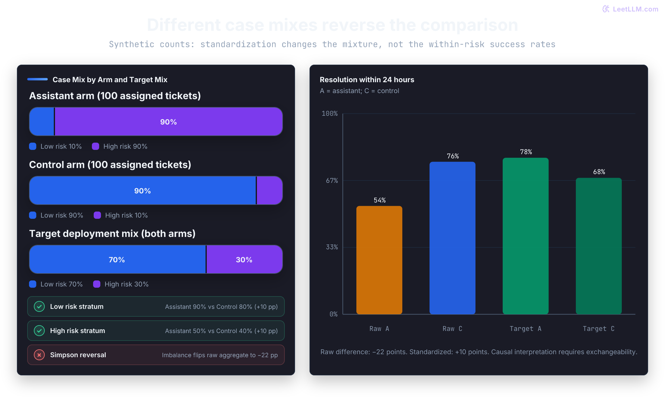
Watch the aggregate reverse the group results
Work with a synthetic log of 200 tickets. Treatment means routing a ticket to a fixed assistant workflow; control means routing it to the existing human workflow. Success means resolution within 24 hours, measured the exact same way in both arms. Risk is recorded before routing, not inferred from the assistant's response.
Within each risk group, the assistant's observed success rate is ten percentage points higher. Before looking at the totals, predict what the aggregate would say if both arms had the same risk mix.
| Ticket risk | Assistant success | Control success | Observed difference |
|---|---|---|---|
| Low | 9/10 = 90% | 72/90 = 80% | +10 percentage points |
| High | 45/90 = 50% | 4/10 = 40% | +10 percentage points |
| Naive aggregate | 54/100 = 54% | 76/100 = 76% | -22 percentage points |
The totals compare different populations. The assistant receives 90 difficult tickets; control receives 90 easy tickets. That unequal mix flips the aggregate direction.
This reversal is Simpson's paradox: group composition changes the direction of the aggregated association. Observational counts alone still don't establish a causal improvement.
The next snippet computes both within-group differences and the reversed aggregate. It reports percentage points, not relative percentage changes: 90% minus 80% is 10 points, whereas the relative increase is 10/80 = 12.5%.
groups = {
    "low": {"assistant": (9, 10), "control": (72, 90)},
    "high": {"assistant": (45, 90), "control": (4, 10)},
}

for risk, counts in groups.items():
    assistant_success, assistant_total = counts["assistant"]
    control_success, control_total = counts["control"]
    difference = assistant_success / assistant_total - control_success / control_total
    print(f"{risk:>4} risk difference: {100 * difference:+.0f} percentage points")

assistant_rate = (9 + 45) / (10 + 90)
control_rate = (72 + 4) / (90 + 10)
print(f"naive aggregate difference: {100 * (assistant_rate - control_rate):+.0f} percentage points")low risk difference: +10 percentage points
high risk difference: +10 percentage points
naive aggregate difference: -22 percentage pointsThe reversal disappears once both workflows are compared against the same risk distribution. That repairs the visible mix, but it still leaves a deeper question: for one assistant-handled ticket, what would control have done?
Pearl's ladder: association, intervention, and counterfactuals
A predictor trained on observational logs can learn without learning what changing would do. Routing and customer selection help determine which examples appear in those logs. Pearl's causal hierarchy separates three kinds of question: association, intervention, and counterfactuals.[2] A system's training objective and causal assumptions matter; “machine learning” doesn't restrict every model to one rung.
Rung 1: association (seeing)
Observational queries ask: Among tickets assigned to the assistant, what fraction resolved? In the log, . This describes the assistant-assigned cases. It combines the workflow's performance, their risk mix, and any other selection or measurement effects; it doesn't isolate the assistant's causal contribution.
Rung 2: intervention (doing)
Interventional queries ask: What fraction would resolve if a specified population were routed to the assistant? Write this as . In a structural causal model, this intervention replaces the equation assigning with and removes its incoming arrows. It leaves the other mechanisms unchanged. Define the population too: our deployment target has 70% low-risk tickets.
Conditioning and intervention generally give different answers under confounding, but their numerical values can coincide through cancellation. The do-notation names the query; it doesn't identify its value from a dashboard. Identification needs a justified causal model or experimental evidence. If routing every ticket changes the shared queue, that effect must be part of the intervention model.
Rung 3: counterfactuals (imagining)
Counterfactual queries combine evidence from the actual world with an alternative action: Given that a control-assigned ticket failed, would it have resolved under the assistant? The corresponding probability is . Conditioning only on those two facts describes a group of failed control tickets; a question about ticket #102 can condition on its other recorded features too.
Even knowing both intervention success rates doesn't determine that counterfactual probability. It needs information about how the two potential outcomes are paired within units. Causal assumptions can help identify or bound such queries; asking an LLM to imagine the alternative doesn't supply the missing evidence.
A dashboard reports 15% higher relative retention among users who choose an LLM code-explanation feature. Does this comparison establish the benefit of offering it to everyone?
Answer
No. Motivation could influence both feature use and retention. Specify the action: offering the feature to everyone and forcing everyone to use it are different interventions. Randomizing the offer can estimate its effect on retention, without automatically identifying the effect of actual feature use.
Separate observed outcomes from missing alternatives
Take one difficult ticket that received the assistant and resolved within 24 hours. Its observed outcome is 1. Define for assistant assignment and for control. The potential outcomes and are that ticket's binary resolution outcomes under the two workflows. Their difference is its individual treatment effect.
At this ticket's original decision point, we observe its outcome under one actual assignment. Here , but the counterfactual could be 0 or 1. The assistant may have caused this success, or the ticket may have resolved either way. Another control ticket can help estimate an average, but doesn't reveal this ticket's missing outcome. Replaying a case later changes its history; a simulated replay answers a question about the simulator. This limitation is the Fundamental Problem of Causal Inference.[3]
These potential outcomes refer to well-defined workflows and the same 24-hour horizon. Record the assistant policy, model and prompt versions, available tools, and control procedure. A stochastic assistant can be a defined policy; consistency doesn't require identical text on every run. The binary response-type example below treats potential outcomes as fixed for each hypothetical ticket.
Causal estimands: ATE and ATT
The average treatment effect averages those individual differences across a specified target population:
For binary resolution, an ATE of 0.10 means ten additional resolutions per 100 tickets on average under assistant assignment versus control.
Engineers also inspect the Average Treatment Effect on the Treated (ATT):
If assignment is independent of potential outcomes with a common treatment probability, these population estimands coincide. A finite randomized run can still have different realized average effects in its treated subset by chance. Risk-dependent randomization doesn't automatically give marginal independence.
With selective routing and heterogeneous effects, ATT can differ from ATE. If difficult tickets benefit more and are overrepresented among treated cases, ATT can exceed the log-population ATE. In our displayed table both estimated subgroup differences are +10 points, so changing the risk mix leaves that estimated difference unchanged.
Latent response types and the counterfactual matrix
Because individual counterfactuals are hidden, every unit in a binary-outcome setting belongs to one of four latent response types:
- Always Resolves (Immune): . The ticket succeeds under either workflow.
- Helped (Beneficiary): . The assistant succeeds where legacy control fails.
- Harmed (Adverse): . Legacy control succeeds, but the assistant fails.
- Never Resolves (Doomed): . The ticket fails under both workflows.
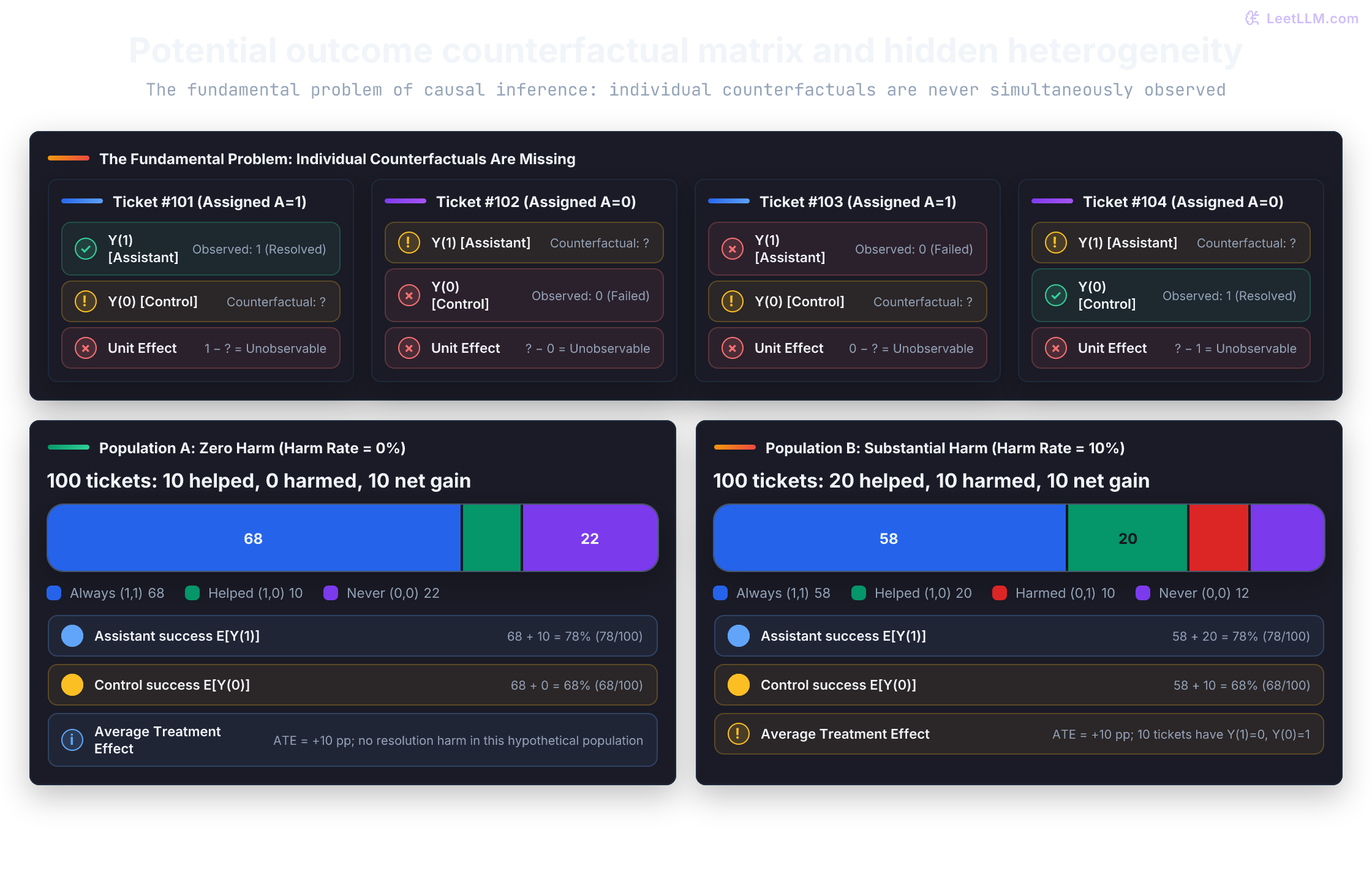
Consider two hypothetical populations of 100 tickets, with both potential outcomes filled in for illustration:
| Potential-outcome type | Population A | Population B | ||
|---|---|---|---|---|
| Resolves under either workflow | 1 | 1 | 68 | 58 |
| Helped by assistant | 1 | 0 | 10 | 20 |
| Harmed by assistant | 0 | 1 | 0 | 10 |
| Resolves under neither | 0 | 0 | 22 | 12 |
Both populations produce 78 assistant successes and 68 control successes. In Population A, ten tickets benefit and zero are harmed. In Population B, twenty benefit and ten are harmed. The net gain is ten points in both cases. Even an ideal randomized experiment identifying both marginal outcome rates can't determine their within-ticket pairing. Under these fixed binary potential outcomes, a no-harm assumption would rule out Population B and identify the proportions of the four types, but not which tickets belong to them. The data's positive average doesn't establish that assumption or safety on other metrics.
The next snippet verifies both populations from their underlying counts:
import numpy as np

# Columns are Y(1), Y(0); rows match the four types in the table.
potential_outcomes = np.array([[1, 1], [1, 0], [0, 1], [0, 0]])
populations = {"A": np.array([68, 10, 0, 22]), "B": np.array([58, 20, 10, 12])}

for name, counts in populations.items():
    rates = counts @ potential_outcomes / counts.sum()
    effect = rates[0] - rates[1]
    print(
        f"{name}: assistant={rates[0]:.0%}, control={rates[1]:.0%}, "
        f"ATE={100 * effect:+.0f} points; helped={counts[1]}, harmed={counts[2]}"
)A: assistant=78%, control=68%, ATE=+10 points; helped=10, harmed=0
B: assistant=78%, control=68%, ATE=+10 points; helped=20, harmed=10Knowing only the exact marginal rates 78% under assistant and 68% under control, what is the largest possible resolution-harm rate in these fixed binary populations?
Answer
22%. Harm requires failure under assistant and success under control, so it can't exceed the 22% who fail under assistant. The counts 46 always resolve, 32 helped, 22 harmed, and 0 never resolve achieve both margins. Zero harm is possible too, as Population A shows. The margins bound harm without identifying it.
Causal graphs, d-separation, and the three canonical junctions
The routing table shows an imbalanced mix, but not why routing produced it. Suppose the triage system sends difficult tickets to the assistant more often. Risk exists before routing and influences both assignment and resolution, making it a confounder.
A causal directed acyclic graph (DAG) records assumed direct causal relationships. It can accompany structural equations, but the graph alone doesn't specify their functions or effect sizes. Arrows aren't correlations inferred from the table. A DAG is acyclic; a feedback system may need variables indexed by time.
d-separation describes path blocking, using three elementary junctions.[3] An open path permits dependence rather than guaranteeing a nonzero association: effects can cancel. Under the causal Markov assumption, d-separation implies conditional independence. Claims in the reverse direction need a faithfulness assumption.
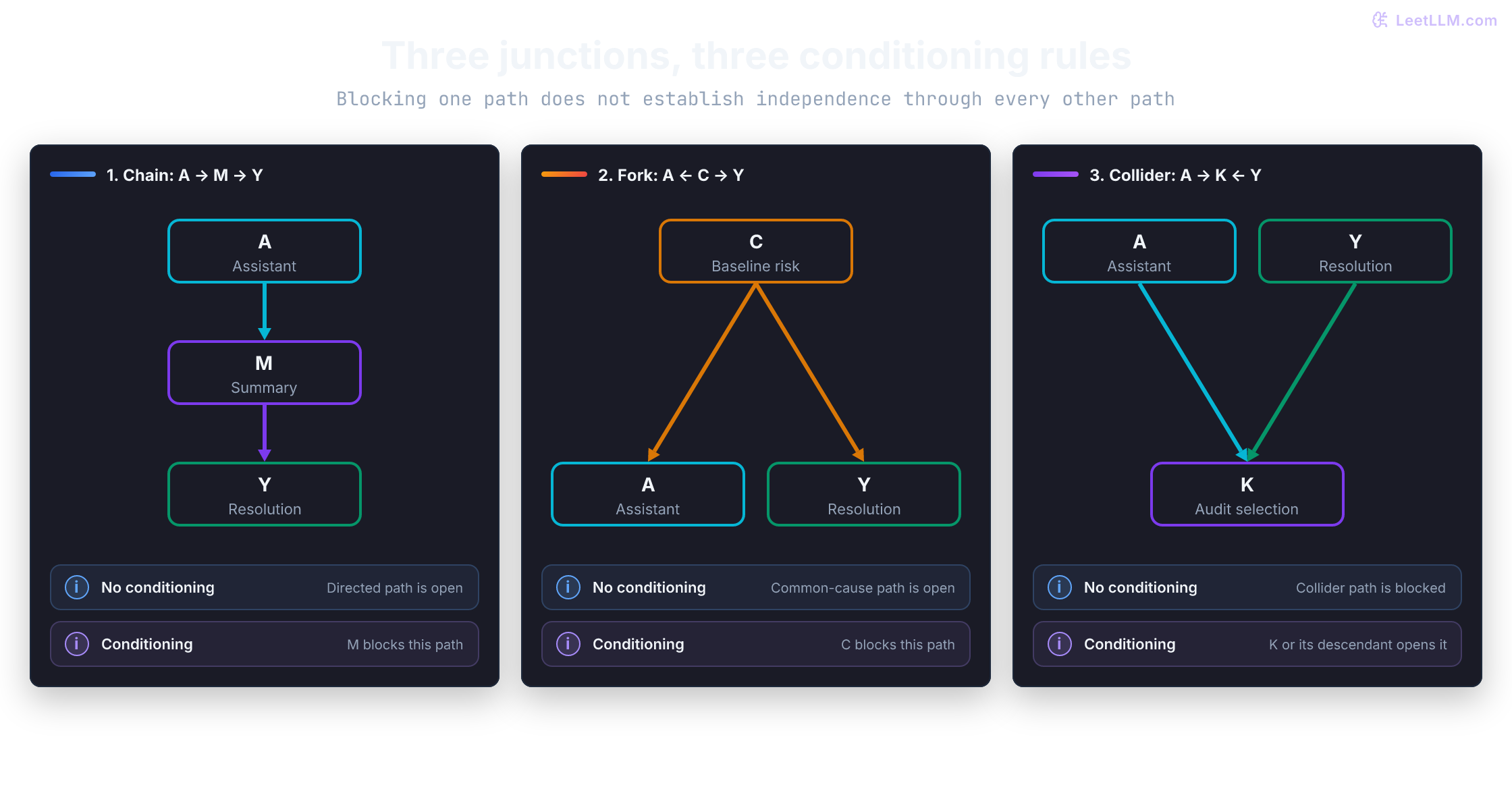
1. The chain (mediator):
In this assumed graph, treatment changes diagnostic summary , which influences resolution .
- Without conditioning, this directed path is open.
- Conditioning on blocks this path. It removes the mediated route from a total-effect comparison.
That operation doesn't automatically identify a direct causal effect. Other paths and mediator-outcome confounding matter, and conditioning on differs from intervening to fix it. The isolated chain shown has no direct arrow.
2. The fork (confounder):
A pre-treatment common cause influences assignment and resolution. Risk can play that role in the triage system.
- Without conditioning, the path is open.
- Conditioning on blocks this backdoor path.
Risk adjustment supports causal identification only if it blocks the relevant noncausal paths and the other identification assumptions hold. The Simpson reversal alone doesn't establish that risk is the only confounder.
3. The collider (inverted fork):
Two arrows meet at their common effect . A variable is a collider on a particular path; the two causes needn't be independent through every other path.
- Without conditioning on or its descendants, this path is blocked.
- Conditioning on , or a descendant of , opens it. Other non-colliders can still block a longer path.
To expose the direction of bias, use a fresh fixture in which assistant assignment has no effect on resolution: each workflow resolves 50 of 100 tickets. Audit a ticket if the assistant was used or it failed, so . All assistant tickets enter the audit, but only control failures enter. Predict the assistant advantage in the filtered log.
# Independent A and Y in this balanced, no-effect fixture.
records = [(a, y) for a in (0, 1) for y in (0, 1) for _ in range(50)]
audited = [(a, y) for a, y in records if a == 1 or y == 0]

for label, subset in (("all tickets", records), ("audited only", audited)):
    rates = {}
    for a in (0, 1):
        outcomes = [y for assigned, y in subset if assigned == a]
        rates[a] = sum(outcomes) / len(outcomes)
    print(
        f"{label}: assistant={rates[1]:.0%}, control={rates[0]:.0%}, "
        f"difference={100 * (rates[1] - rates[0]):+.0f} pp"
)all tickets: assistant=50%, control=50%, difference=+0 pp
audited only: assistant=50%, control=0%, difference=+50 ppFiltering creates a positive association between assistant use and successful resolution in this example. An arrow doesn't specify a positive effect: success suppresses the failure-triggered audit. Different audit rules can produce a different sign. This is selection bias, not evidence that the assistant helps.
The backdoor criterion
The backdoor criterion gives a sufficient graphical condition for an adjustment set :[3]
A covariate set satisfies the backdoor criterion for when no member is a descendant of and conditioning on blocks every path from to that starts with an arrow into .
For a causal model represented by that DAG, with consistency and positivity over the target support, this sufficient criterion licenses adjustment:
Ticket risk is recorded before routing, while an escalation note is created by the assistant after routing. Which variable can support backdoor adjustment, and why can't the other replace it?
Answer
Risk can block the common-cause fork under the assumed graph. The assistant-generated note is treatment-affected, so using it as a baseline adjustment can remove mediated effects or induce selection bias. Recording a variable later doesn't alone make it treatment-affected; its causal role matters.
Standardize both arms to one population
Suppose the planned deployment has 70% low-risk and 30% high-risk tickets. What would each workflow's resolution rate be at that same mix? The assistant rate becomes ; the control rate becomes . Their standardized difference is:
The hat marks an estimate from observed data. Both within-group differences are ten points, so this weighted difference is ten points for any shared risk mix. The individual arm rates depend on the mix, and unequal subgroup differences would make the estimated effect depend on it too. Calling this difference an identified causal effect requires explicit identification conditions.[3]
The next snippet continues the earlier session and applies one shared population distribution to both arms:
target_weights = {"low": 0.7, "high": 0.3}
standardized = {"assistant": 0.0, "control": 0.0}

for risk, population_weight in target_weights.items():
    for workflow in standardized:
        successes, total = groups[risk][workflow]
        standardized[workflow] += population_weight * successes / total

adjusted_effect = standardized["assistant"] - standardized["control"]
for workflow, rate in standardized.items():
    print(f"{workflow} at the target mix: {rate:.0%}")
print(f"standardized difference: {100 * adjusted_effect:+.0f} percentage points")
assert abs(adjusted_effect - 0.10) < 1e-12assistant at the target mix: 78%
control at the target mix: 68%
standardized difference: +10 percentage pointsThe arithmetic answers a target-population comparison. It estimates an identified causal effect only under explicit assumptions:
| Identification assumption | Meaning in the ticket example |
|---|---|
| Conditional exchangeability | Within measured risk groups, no unrecorded common cause still changes both routing and resolution: . |
| Positivity or overlap | Both assistant and control assignments occur for every target risk stratum: . |
| Consistency | Treatment policies are well-defined and the outcome matches the policy received: . |
| No interference | One ticket's assignment doesn't alter another's outcome, such as through queue spillover. Together with no consequential hidden treatment versions, this is the usual SUTVA requirement. |
| Transfer to target | The 70% and 30% weights describe deployment, and risk-specific potential-outcome averages apply there too. |
The smallest strata contain only ten tickets. If one low-risk assistant success became a failure, its rate would fall from 90% to 80%, and the standardized difference would fall from ten points to three. That's a sensitivity check, not a formal confidence interval.
How uncertain is the +10-point standardized difference? For independent tickets, fixed target weights, and a conditional binomial model within each workflow/risk cell, a rough plug-in calculation adds the stratum variances with squared weights:
from math import sqrt

variance_of_difference = 0.0
for risk, weight in target_weights.items():
    for workflow in ("assistant", "control"):
        successes, total = groups[risk][workflow]
        rate = successes / total
        variance_of_difference += weight**2 * rate * (1 - rate) / total

se = sqrt(variance_of_difference)
low, high = adjusted_effect - 1.96 * se, adjusted_effect + 1.96 * se
print(f"plug-in standard error: {100 * se:.2f} pp")
print(f"rough normal interval: [{100 * low:.1f}, {100 * high:.1f}] pp")plug-in standard error: 8.77 pp
rough normal interval: [-7.2, 27.2] ppThe point estimate looks promising, but these few tickets leave broad uncertainty. This normal approximation can have poor coverage with sparse cells such as 9/10; select an interval method suitable for the sampling design before making a claim. Clustering or estimated deployment weights need additional uncertainty treatment. More data reduce sampling variance under a sound design; they don't remove unmeasured confounding.
Both observed risk groups show a ten-point advantage, but within each risk group a hidden customer-tier field affects both routing and resolution. Does standardizing only by recorded risk identify the causal effect?
Answer
Not necessarily. The arithmetic still returns a risk-adjusted ten-point association, but an unmeasured common cause violates conditional exchangeability. Without measuring and adjusting for customer tier, or switching to a randomized design, that association isn't guaranteed to be causal.
Weight the assignment, then check its support
Standardization averages group-specific outcomes at a chosen mix. Inverse Probability of Treatment Weighting (IPTW) instead weights each observation by the inverse of the probability of receiving the treatment it actually received. The propensity score is the conditional assignment probability , not the probability of successful resolution.[3]
Estimate it from the log: low-risk tickets went to the assistant 10 times out of 100, so . High-risk tickets went 90 times out of 100, so . An assistant ticket gets weight ; a control ticket gets .
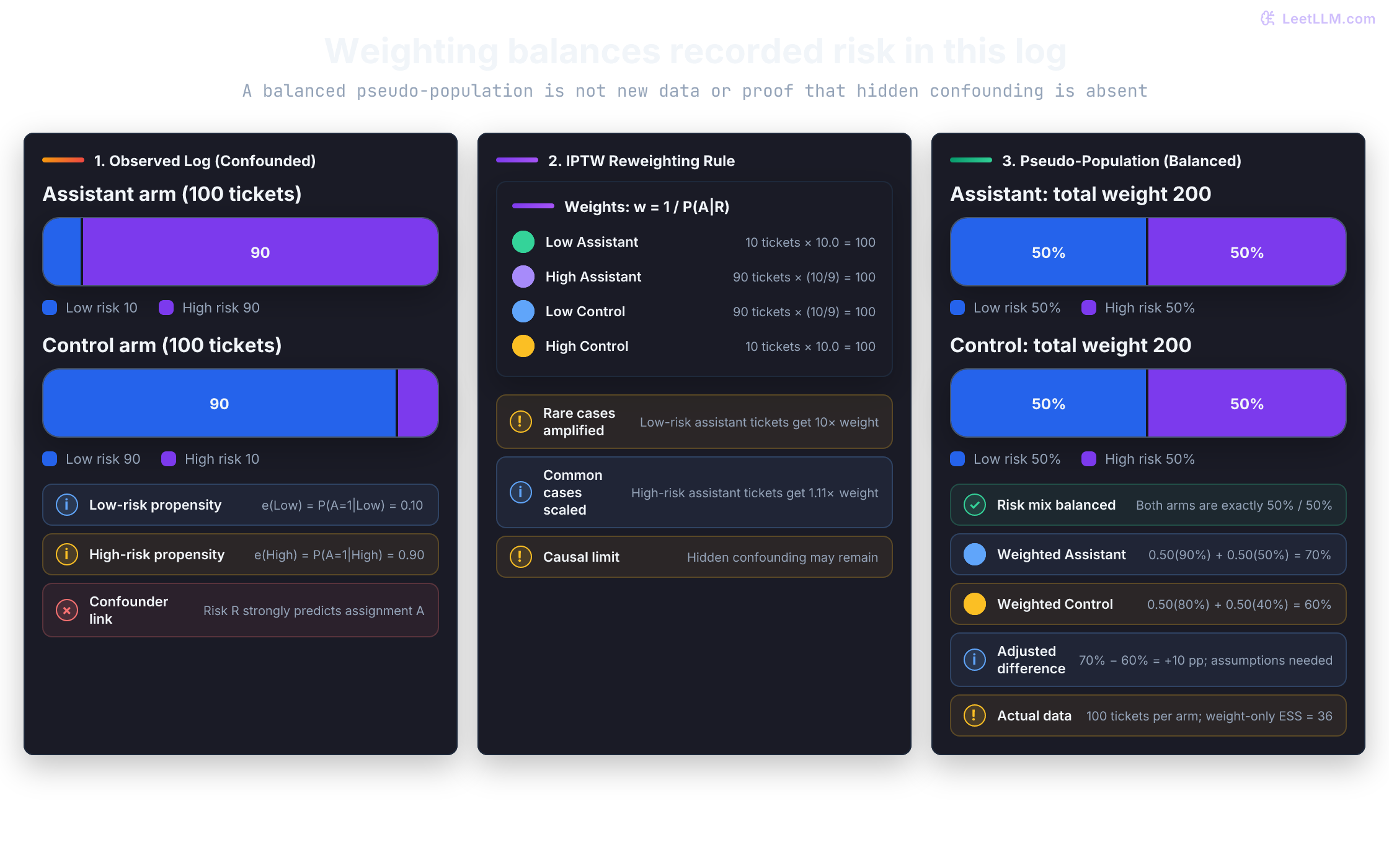
The ten low-risk assistant tickets each get weight 10, for total weight 100. The ninety high-risk assistant tickets each get weight , also totaling 100. The control arm gets the same 100/100 weighted mix. These weights recover the logged population's 50%/50% risk mix, not the planned deployment's 70%/30% mix. Weighting and standardization agree when they target the same population.
This snippet works directly with the grouped counts:
import numpy as np

totals = np.array([[10, 90], [90, 10]], dtype=float)
successes = np.array([[9, 72], [45, 4]], dtype=float)

def assignment_weights(counts):
    if np.any(counts <= 0):
        raise ValueError("No within-risk comparison: a workflow has zero tickets")
    propensity = counts[:, 0] / counts.sum(axis=1)
    return propensity, np.column_stack([1 / propensity, 1 / (1 - propensity)])

propensity, weights = assignment_weights(totals)
weighted_totals = totals * weights
rates = (successes * weights).sum(axis=0) / weighted_totals.sum(axis=0)
print("assignment propensity (low, high):", propensity)
print("weighted counts, rows=low/high; columns=assistant/control:")
print(np.round(weighted_totals, 1))
print(f"50/50 mix: assistant={rates[0]:.0%}, control={rates[1]:.0%}")
print(f"weighted difference: {100 * (rates[0] - rates[1]):+.0f} percentage points")
effective_n = weighted_totals.sum(axis=0)**2 / (totals * weights**2).sum(axis=0)
print("weight-only ESS diagnostic (assistant, control):", np.round(effective_n, 1))

try:
    assignment_weights(np.array([[10, 90], [100, 0]]))
except ValueError as error:
print("unsupported comparison:", error)assignment propensity (low, high): [0.1 0.9]
weighted counts, rows=low/high; columns=assistant/control:
[[100. 100.]
[100. 100.]]
50/50 mix: assistant=70%, control=60%
weighted difference: +10 percentage points
weight-only ESS diagnostic (assistant, control): [36. 36.]
unsupported comparison: No within-risk comparison: a workflow has zero ticketsPositivity violations and extreme weights
If the routing policy always sends high-risk tickets to the assistant, . That is a structural positivity violation for a target effect comparing both workflows on high-risk tickets. Weighting can't recover the missing control rate. Restrict the target to supported cases, collect exploration data, or disclose the extra assumptions used to extrapolate.
A zero cell in a finite sample doesn't by itself prove that the underlying assignment probability is zero. It can occur by chance even with a supported policy. The snippet rejects direct within-stratum arithmetic on either kind of empty cell rather than silently extrapolating.[3]
Near-zero probabilities can still make estimates unstable: an assignment probability of 0.005 gives weight 200. Our pseudo-counts total 200 per arm, but each arm has only 100 tickets. A common weight-only diagnostic is ; here it's just 36 per arm. This diagnoses weight concentration, not an exact outcome-specific variance or a confidence interval.
Three choices are often confused:[3]
- Hájek normalization estimates an arm mean as , as the code does. It's a ratio estimator, generally not exactly unbiased in finite samples.
- Stabilized weights use a numerator such as . Here the numerator is 0.5 in each arm. That constant cancels in a normalized arm mean, leaving the same estimate and weight concentration.
- Clipping weights caps large values and can trade variance for bias. The bias needn't be small, and the cap changes the effective weighted comparison. Predeclare it and examine sensitivity.
Check balance and support after fitting a propensity model. A misspecified model needn't balance measured covariates in a finite sample. Neither normalization nor stabilization repairs unmeasured confounding or unsupported actions.
The weighted assistant rate is 70%, while the 70/30 standardized assistant rate was 78%. Did one calculation fail?
Answer
No. The inverse-probability weights here target the log's 50/50 risk mix: 0.5(0.90) + 0.5(0.50) = 0.70. Deployment standardization targets 70/30: 0.7(0.90) + 0.3(0.50) = 0.78. The differences between arms happen to agree because both risk groups share the same ten-point difference.
Instrumental variables when unmeasured confounders lurk
Suppose hidden urgency leaves an open common-cause path even after risk adjustment. Conditional exchangeability given risk then fails under the assumed graph. Risk-only standardization and IPTW don't remove this residual confounding. An unrecorded variable doesn't necessarily cause residual confounding if the recorded adjustment set already blocks its relevant paths.
An instrumental variable (IV) offers another identification route, with demanding assumptions. For our binary randomized encouragement , first justify:[3]
- Relevance: changes the probability of receiving the assistant. The first-stage difference is nonzero.
- Exclusion: Changing has no effect on a ticket's resolution except through the workflow it receives. Removing a direct arrow is insufficient if another bypassing path remains.
- Independence: Randomized is independent of potential workflow uptake and outcomes. Independence from one named confounder alone wouldn't establish this.
Also define the instrument and workflows consistently and address interference. Checking the first stage doesn't prove exclusion or independence.
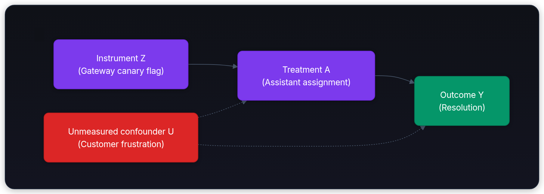
Consider an invisible randomized gateway encouragement that changes only the chance of assistant routing. Treat its validity as a design assumption to audit. A latency experiment is a poor substitute: delay can change resolution directly even if it doesn't change customer frustration. A canary flag that also changes model versions, timeouts, or staff behavior has the same exclusion problem.
Wald estimator and local average treatment effects
With binary instrument and workflow uptake, the Wald ratio divides the outcome difference across instrument groups by their workflow-uptake difference. Hats emphasize that sample means produce an estimate:
Suppose setting canary flag raises assistant usage from 30% to 70% (), while overall ticket resolution rises from 68% to 72% (). The Wald estimate is:
Under the instrument assumptions and monotonicity, for every ticket, the population ratio identifies the local average treatment effect (LATE) on compliers: tickets with .[3] No defiers means encouragement never makes a ticket receive control when it would otherwise receive the assistant. It doesn't mean every ticket follows the encouragement.
The example allows assistant use at 30% even under , so it isn't one-sided noncompliance. Under monotonicity, the uptake rates imply 30% always-takers, 40% compliers, and 30% never-takers. LATE can apply with this two-sided noncompliance; it needn't equal the whole-population ATE. Another instrument may move a different subset.
A small first-stage denominator makes the ratio unstable and magnifies exclusion violations. Estimate uncertainty for the ratio with a method appropriate to instrument strength. The displayed numbers are a hypothetical calculation, not evidence that our gateway flag is valid.
Why can't an engineer use the ticket's word count as an instrument for assistant routing?
Answer
If complexity affects both word count and resolution, word count has a common-cause path to the outcome, violating independence. If changing word count also affects resolution outside routing, exclusion fails too. Being associated with assistant use isn't enough to make a variable a valid instrument.
Causal inference in production AI systems
Causal principles are fundamental to machine learning and AI agent engineering, particularly when models interact with environments, user behavior, and multi-step tool calls.
Offline policy evaluation (OPE)
For a one-step routing policy , offline policy evaluation estimates its value from contexts, actions, and rewards logged under .[4] Here is pre-routing risk and chooses between the two fixed workflows. The target policy can choose the assistant more often without changing what “assistant” means.
This requires supported target actions, observed context sufficient for unconfounded action selection, consistent action/reward definitions, and stable relevant mechanisms. A new prompt that changes the assistant's behavior is a new action version; logs of the old workflow don't automatically identify its value. The inverse-propensity estimator (IPS) weights logged rewards by the policy ratio:
For a multi-step trajectory, an importance ratio can involve , where records the relevant history. Under suitable assumptions, trajectory-wise or per-decision weighting accounts for changed action and state distributions. Variance can grow exponentially with horizon, but isn't guaranteed to do so; identical policies give ratio 1.[5]
Return to one-step routing. A doubly robust (DR) estimator combines a reward model with a weighted residual. Define :
Why two models? Let be the true logging propensity, its estimate, and the true conditional reward mean. For fixed nuisance models evaluated on independent data, the conditional bias is:
It vanishes if either model is exactly correct on the supported target actions.[4] With estimated models, correct specification and consistent fitting can give consistency under suitable regularity conditions; they're not automatic exact finite-sample unbiasedness. Split data or cross-fit nuisance models, evaluate a learned target policy on held-out data, and use suitable uncertainty. Neither model substitutes for causal identification or overlap.
The formula above is for a one-step contextual bandit. A multi-step agent needs a sequential estimator with future value and per-step corrections; applying this immediate-reward formula to every tool call doesn't evaluate its trajectory return.[5]
The next snippet reconstructs the 200 observed tickets. Its “matched” models reproduce the empirical stratum rates and assignment fractions. Predict whether the residual correction repairs the deliberately shifted reward model when the propensity also misses the risk-dependent routing. Exact agreement in this grouped fixture verifies algebra, not repeated-sample unbiasedness or causal identification.
import numpy as np

# Reconstruct individual records from the 200 tickets
# Stratum: risk (0: low, 1: high), action A (1: assistant, 0: control), outcome Y
records = []
records.extend([(0, 1, 1)] * 9 + [(0, 1, 0)] * 1)    # Low assistant: 9/10
records.extend([(0, 0, 1)] * 72 + [(0, 0, 0)] * 18)  # Low control: 72/90
records.extend([(1, 1, 1)] * 45 + [(1, 1, 0)] * 45)  # High assistant: 45/90
records.extend([(1, 0, 1)] * 4 + [(1, 0, 0)] * 6)    # High control: 4/10

data = np.array(records)
risk, a_obs, y_obs = data[:, 0], data[:, 1], data[:, 2]

# Empirical logging fractions for assistant assignment.
pi_0 = np.where(risk == 0, 0.10, 0.90)

# Evaluate candidate policy pi_target: always route to assistant (action 1)
pi_target = 1.0
w = np.where(a_obs == 1, pi_target / pi_0, 0.0)

# Reward model deliberately shifted from the observed stratum rates.
matched_q_1 = np.where(risk == 0, 0.90, 0.50)
q_hat_1 = matched_q_1 + 0.05
q_hat_obs = np.where(a_obs == 1, q_hat_1, 0.50)

v_ips = np.mean(w * y_obs)
v_direct = np.mean(q_hat_1)
v_dr = np.mean(q_hat_1 + w * (y_obs - q_hat_obs))

print(f"Direct model (+5 pp): {v_direct:.1%}")
print(f"IPS (matched routing): {v_ips:.1%}")
print(f"DR (matched routing, shifted reward): {v_dr:.1%}")

wrong_weights = np.where(a_obs == 1, 1 / 0.40, 0.0)
matched_q_obs = np.where(a_obs == 1, matched_q_1, 0.50)
dr_matched_reward = np.mean(matched_q_1 + wrong_weights * (y_obs - matched_q_obs))
dr_both_wrong = np.mean(q_hat_1 + wrong_weights * (y_obs - q_hat_obs))
print(f"DR (wrong routing, matched reward): {dr_matched_reward:.1%}")
print(f"DR (both models wrong): {dr_both_wrong:.1%}")
assert abs(v_dr - 0.70) < 1e-12Direct model (+5 pp): 75.0%
IPS (matched routing): 70.0%
DR (matched routing, shifted reward): 70.0%
DR (wrong routing, matched reward): 70.0%
DR (both models wrong): 68.8%The matched-model results target the log's 50/50 risk mix: 70% assistant resolution. They aren't the 78% value at the separate deployment mix. The two wrong models leave a weighted-residual error here; double robustness doesn't protect against their simultaneous failure. This is still an adjusted association unless the identification assumptions hold.
When possible, log the actual action probability and policy version at each decision rather than infer them from aggregate counts. Include eligibility, reward windows, missing outcomes, and relevant context. If a hidden urgency score drives both action and reward, a propensity fitted only to displayed risk doesn't restore exchangeability.
Recommendation and search debiasing
Search clicks reflect exposure as well as relevance. Under the simple position-based model, an item is clicked only if it's examined and relevant. Then under the model's independence assumptions. Joachims et al. use observation propensities to correct a ranking objective.[6]
Position is part of the presentation mechanism; calling it a confounder isn't itself a justification for weighting. Estimate and validate the examination or click model, ensure positive observation probabilities, and account for violations such as trust or attractiveness effects. Correcting position bias under that model doesn't automatically recover all “true preferences” or remove popularity and selection bias.
Counterfactual reasoning in LLM agents
When an autonomous agent executes a sequence of tool calls (e.g. database query, code generation, test execution) and fails at step 5, diagnosing which step caused the failure is non-trivial. Did tool call 2 return subtly corrupted data, or did tool call 4 fail on valid input?
A trace's order isn't a causal DAG by itself. State, tool results, random choices, and environment changes determine downstream behavior. In a controlled replay, snapshot the environment before call 2, replace its return value, and rerun later steps with a declared randomness policy. Recompute downstream state that depends on the replaced result; freezing it would block the mechanism being tested.
Paired replays can measure the effect of that replacement inside the replay environment. Match or repeat random draws, prevent outside state drift, and specify the alternative result. Intervening on a tool's return value differs from changing its implementation, including its side effects. One successful replay doesn't prove the historical root cause or provide uniquely identified reinforcement-learning credit. Those conclusions need a justified causal model and a clear estimand.[2]
Decide what the comparison supports
| Evaluation method | Identification requirements | Core advantages | Primary failure modes |
|---|---|---|---|
| Standardization (g-formula) | Exchangeability, positivity, consistency, suitable conditional-outcome estimation | Direct estimation across target population distributions | Unmeasured confounding; outcome estimation errors |
| Inverse Weighting (IPTW) | Exchangeability, positivity, consistency, justified propensity estimation | Targets an adjusted comparison without fitting outcome means | Hidden confounding, concentrated weights, unsupported actions |
| Instrumental Variables (IV) | Relevance, independence, exclusion, consistency, non-interference; monotonicity for this LATE | Can identify a complier effect despite treatment-outcome confounding | Invalid or weak instrument; complier effect may not transfer to everyone |
| Doubly Robust (one-step DR / OPE) | Identification and overlap; consistent fitting of at least one nuisance model with suitable regularity | Two chances to control model error; can improve precision | Both models wrong, weak overlap, invalid causal assumptions, evaluation leakage |
| Randomized A/B experiment | Known randomization, well-defined policies, suitable outcome measurement and interference model | Assignment needn't depend on baseline potential outcomes | Queue interference, missing outcomes, limited external validity, no individual pairing |
A marginally randomized design makes assignment independent of potential outcomes; a conditionally randomized design does so conditional on its randomization strata. Baseline arm balance holds in expectation, not exactly in every realized sample. Neither design automatically repairs missing outcomes, interference, or measurement errors. For tickets sharing an agent pool, assigning one to the assistant can free staff time for another. Define whether you want an individual routing effect, a queue-level policy effect, or another estimand, then design the comparison accordingly.
For this release report, the raw -22-point difference compared unequal case mixes. The +10-point standardized difference addresses the visible imbalance, but needs an uncertainty calculation and credible identification and transfer assumptions before supporting deployment. It doesn't prove every ticket benefited. A well-run randomized evaluation can address routing confounding for its defined population; validate outcomes and queue effects too.
Before recommending a rollout, write a short evidence receipt: target population, two workflow definitions, resolution horizon, routing probabilities, adjustment set and causal graph, overlap diagnostics, effect with uncertainty, missing-outcome handling, and queue/interference assumptions. Mark each claim as observed, identified under assumptions, or unresolved. That's the useful next artifact from this 200-ticket log.