Accelerator Architecture Field Guide

An 8-billion-parameter code assistant receives eight repository prompts, each 4,096 tokens long. It ingests the prompts in a flash, yet stumbles when generating its answers token by token. A chip advertised with double the peak arithmetic per second sounds tempting, but it might leave generation speed almost completely unchanged. What is the machine actually waiting for?

The CUDA foundation introduced kernels, thread blocks, warps, device memory, and synchronized timing. The model-parallelism lesson demonstrated that a logical shard count isn't a physical route. Keep both ideas: an accelerator runs work through a concrete execution hierarchy, and every tensor or collective travels through a concrete physical memory path.

One projection, two different machines inside it

Use an illustrative feed-forward projection for the assistant, not the specifications of a named 8B checkpoint. Each input row has K = 4,096 features, and the projection produces N = 11,008 features. Its simplified matrix multiplication is:

M is the number of token rows processed together. BF16 stores each matrix element in 2 bytes. The weight matrix contains about 86 MiB, independent of phase.

During prefill, prompt positions can be processed together. Assume the scheduler puts all eight 4,096-token prompts into this projection at once, giving M = 32,768. Chunked prefill would use smaller groups. During ordinary one-token decode, each active sequence contributes one new token, so the same eight requests give M = 8. The weight shape hasn't changed. Reuse has.

One output element combines 4,096 products. Counting a multiply and an add as two floating-point operations (FLOPs), one row costs about 2 × 4,096 × 11,008 = 90,177,536 FLOPs. For M rows:

For an isolated operation with cold inputs and a materialized BF16 output, count each input and weight read once and each output write once:

Dividing work by traffic gives arithmetic intensity, measured in floating-point operations per byte. The script computes both phases as a shape calculation, not a hardware benchmark.

K = 4_096
N = 11_008
bytes_per_value = 2  # BF16

phases = {
    "prefill": 8 * 4_096,
    "decode": 8,
}

weight_mib = K * N * bytes_per_value / 2**20
print(f"weight matrix: {weight_mib:.0f} MiB")

for phase, rows in phases.items():
    flops = 2 * rows * K * N
    traffic = bytes_per_value * (rows * K + K * N + rows * N)
    intensity = flops / traffic
    print(f"{phase:7s}: M={rows:6,d}, ideal intensity={intensity:7.1f} FLOP/byte")

weight matrix: 86 MiB
prefill: M=32,768, ideal intensity= 2736.0 FLOP/byte
decode : M=     8, ideal intensity=    8.0 FLOP/byte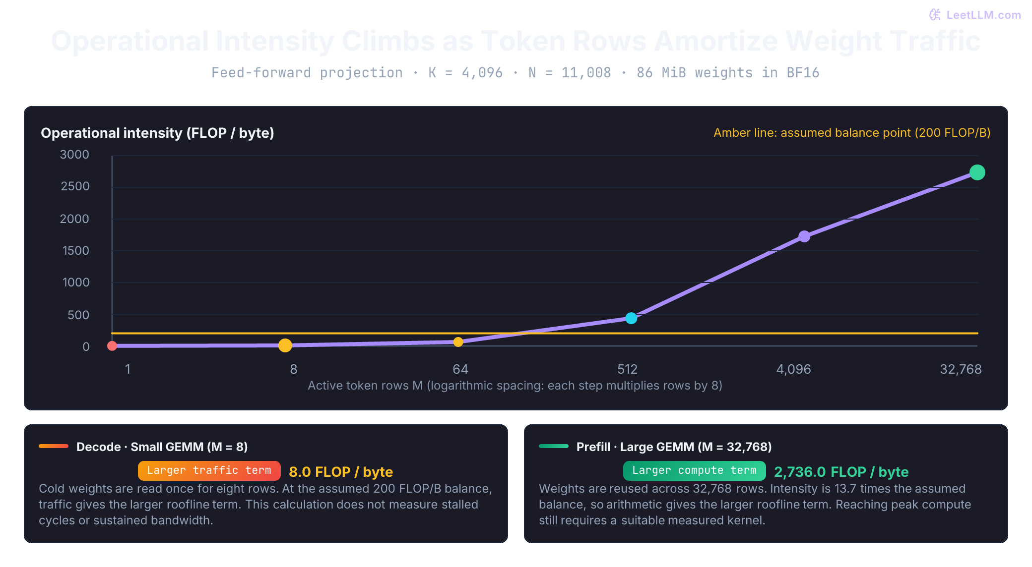

Real kernels reread some tiles, reuse caches, fuse away intermediate writes, and may use quantized weights. The count isn't a measured HBM traffic total or a universal lower bound across fused operations. In the unfused model, prefill presents much more arithmetic per byte than low-concurrency decode. Whether either phase reaches a hardware limit still needs a second number: the machine's compute-to-bandwidth ratio.

Compare work and traffic before predicting time

Consider a hypothetical device with a 200 TFLOP/s compute ceiling and a 1 TB/s memory ceiling for this operation. These are exercise inputs, not a vendor specification or measured rates. Its balance point is 200 FLOP/byte. Below that intensity, the traffic term is larger; above it, the arithmetic term is larger. This is the basic roofline model.^{[1]Reference 1Roofline: An Insightful Visual Performance Model for Multicore Architectureshttps://doi.org/10.1145/1498765.1498785}

For work $F$, bytes $Q$, compute rate $P$, and bandwidth $B$, the optimistic time is:

The maximum assumes perfect overlap. It leaves out launch overhead, synchronization, contention, and work outside this projection. Predict which term wins before running this CPU-only calculation.

K, N = 4_096, 11_008
compute_flops_s = 200e12
bandwidth_bytes_s = 1e12

for phase, rows in [("prefill", 32_768), ("decode", 8)]:
    work = 2 * rows * K * N
    traffic = 2 * (rows * K + K * N + rows * N)
    compute_ms = 1_000 * work / compute_flops_s
    memory_ms = 1_000 * traffic / bandwidth_bytes_s
    term = "compute" if compute_ms > memory_ms else "memory"
    floor_ms = max(compute_ms, memory_ms)
    print(f"{phase}: compute={compute_ms:.3f} ms, memory={memory_ms:.3f} ms, "
          f"floor={floor_ms:.3f} ms ({term})")

prefill: compute=14.775 ms, memory=1.080 ms, floor=14.775 ms (compute)
decode: compute=0.004 ms, memory=0.090 ms, floor=0.090 ms (memory)

Doubling only the compute ceiling halves the prefill floor here but leaves the decode floor unchanged. That isn't a measured speedup. A real kernel can sit far below either ceiling, and a full decode step also reads KV cache, runs other layers, and may exchange collective messages. Long context, higher concurrency, speculative decoding, and cache residency can change which resource dominates.

Memory paths: capacity belongs to an owner

Local storage offers fast access to small live tiles; large memory holds the model and its histories. These aren't interchangeable capacities, and every access doesn't pass through every tier. Registers, shared memory, caches, and explicit DMA buffers have different owners and routes.

Use H100 as one concrete reference rather than assigning one latency table to five architectures:^{[2]Reference 2NVIDIA Hopper Tuning Guidehttps://docs.nvidia.com/cuda/archive/13.0.0/hopper-tuning-guide/index.html[3]Reference 3H100 GPUhttps://www.nvidia.com/en-us/data-center/h100/}

The tuning guide's older HBM summary says up to 3 TB/s; the current product table specifies 3.35 TB/s for H100 SXM. The product's PCIe SKU has different memory and interconnect specifications. Record the SKU with any number you reuse.

How much offload is enough to hurt?

For a deliberately simple traffic exercise, stream 16 decimal GB of dense BF16 weights once per decode batch. Assume 3.35 TB/s for resident reads and a rounded 64 GB/s host path. The second rate is an optimistic exercise input, not a measured PCIe payload rate. Count the two portions sequentially, without overlap, and ignore computation, KV reads, and launch overhead.

weight_bytes = 16e9
resident_rate = 3.35e12
host_rate = 64e9
baseline_s = weight_bytes / resident_rate

for fraction in [0.0, 0.01, 0.10, 1.0]:
    resident_s = weight_bytes * (1 - fraction) / resident_rate
    host_s = weight_bytes * fraction / host_rate
    traffic_s = resident_s + host_s
    print(f"host weights={fraction:4.0%}: traffic={traffic_s * 1000:6.1f} ms, "
          f"ratio={traffic_s / baseline_s:4.1f}x, "
          f"host share={host_s / traffic_s:5.1%}")

host weights=  0%: traffic=   4.8 ms, ratio= 1.0x, host share= 0.0%
host weights=  1%: traffic=   7.2 ms, ratio= 1.5x, host share=34.6%
host weights= 10%: traffic=  29.3 ms, ratio= 6.1x, host share=85.3%
host weights=100%: traffic= 250.0 ms, ratio=52.3x, host share=100.0%

The rate ratio is 52.3, but offloading 1% of weights doesn't imply 98% idle cycles. Even the printed host share is a share of modeled transfer time, not a GPU stall counter. Prefetch, caching, compression, compute overlap, and a larger batch can change the outcome. Dense layers ordinarily consume their weights once for a batch of rows, not separately for every stream; MoE reads depend on the experts selected across that batch.

Residency can avoid repeated host transfers. Offload can still be a useful capacity tradeoff when the resulting latency meets the application's target. Account for recurrent state and any designed KV offload too, rather than declaring all offload impossible.

Thread execution and matrix dataflow

SIMT describes how a group of threads executes instructions. A systolic array describes how matrix operands and partial sums move through arithmetic cells. They answer different questions; a GPU's SIMT programming model doesn't determine every wire inside its matrix engine. Both can support the matrix multiply-accumulate operation:

SIMT warps and matrix cores

An NVIDIA warp has 32 threads; an AMD CDNA wavefront has 64. For ordinary lane-wise arithmetic, active lanes execute the group instruction on their own operands and registers. Divergence and predication determine which lanes participate; lane-local values don't imply independently scheduled instructions.^{[4]Reference 4CUDA Programming Guide.https://docs.nvidia.com/cuda/cuda-programming-guide/[5]Reference 5Introduction to the HIP Programming Modelhttps://rocm.docs.amd.com/projects/HIP/en/develop/understand/programming_model.html}

Matrix multiplication uses specialized units: Tensor Cores on NVIDIA and Matrix Cores on AMD. Threads coordinate to issue operations such as warp-level mma.sync or Hopper warp-group wgmma. Hopper's warp group contains 128 threads. Depending on the instruction variant, the A operand comes from registers or shared memory, the B operand comes from shared memory, and accumulators occupy registers. Shared-memory operand delivery reduces some register movement; it doesn't eliminate register pressure.^{[6]Reference 6Parallel Thread Execution ISAhttps://docs.nvidia.com/cuda/parallel-thread-execution/}

The SM or CU also supports scalar, vector, and reduction work used by normalization, rotary embeddings, and sampling. Those operations use suitable execution units and scheduled instructions. Flexibility doesn't guarantee that every unit stays busy or that switching between kernels has no cost.

Systolic arrays

Google's TPU matrix units and Trainium's tensor engines use systolic matrix dataflow. Neighboring processing elements pass operands or partial sums through the array, avoiding a trip to large memory for each multiply.^{[7]Reference 7An In-Depth Look at Google's First Tensor Processing Unithttps://cloud.google.com/blog/products/ai-machine-learning/an-in-depth-look-at-googles-first-tensor-processing-unit-tpu[8]Reference 8NeuronCore-v3 Architecturehttps://awsdocs-neuron.readthedocs-hosted.com/en/v2.29.1/about-neuron/arch/neuron-hardware/neuron-core-v3.html} The following is a conceptual weight-stationary layout, not a specification of v6e's internal tile geometry.

In a weight-stationary systolic array, weights from matrix $B$ are preloaded into PE registers and remain stationary throughout computation. Activations from matrix $A$ stream in from the left boundary, with rows staggered by one clock cycle so products align correctly. As activations flow horizontally, each PE computes its product, adds it to the incoming partial sum from above, and passes the updated sum downward.

Local operand reuse can make dense matrix products efficient. Array dimensions, fill and drain time, padding, and reduction length still affect useful work. If a hypothetical kernel pads eight useful rows to a 128-row tile, only 8/128 = 6.25% of that tile's rows carry useful values. That arithmetic doesn't establish 93.75% chip idle time: mapping, batching, concurrent work, and other execution engines matter. TPU and Trainium also have vector and scalar resources; their non-matrix work needn't run on the matrix array.

The invariant behind every accelerator

Fast accelerator code keeps reused data close to compute, performs enough work before eviction, and overlaps the next transfer with current arithmetic. Vendor names differ, but four ownership questions don't:

1. Which group executes one instruction together?
2. Which memory can that group share at low latency?
3. Who schedules movement between large memory and local memory?
4. Which physical link carries bytes when work spans devices?

Time to first token (TTFT) measures from request submission to the first returned token, including queueing and any transport within the measurement boundary. Time per output token (TPOT) commonly averages the subsequent generation interval over output_tokens - 1; inter-token latency measures individual gaps. Report the convention, since p95 of request-average TPOT can hide isolated long pauses.

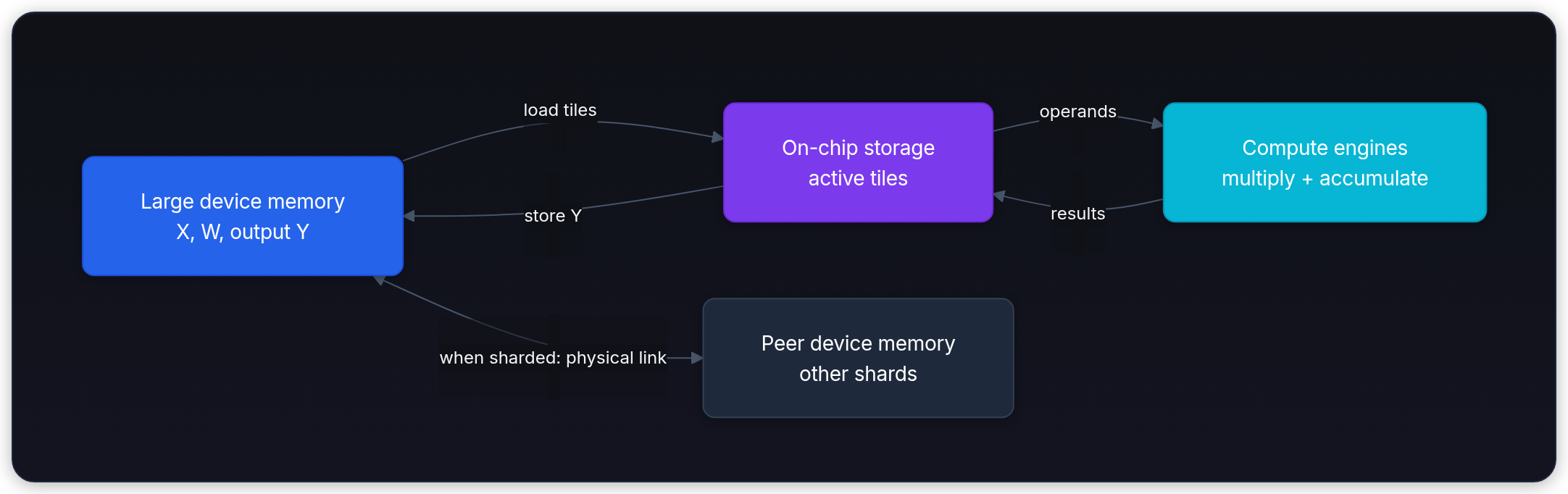
For a tiled projection, large memory supplies input and weight tiles, on-chip storage holds the active pieces, and compute consumes them. Results travel back in the opposite direction. The arrows below describe data movement, not a promise that all platforms expose identical memory instructions.

A platform port is incomplete until latency and output checks use the same prompt distribution. Holding the graph constant doesn't hold its execution path constant.

Documentation boundary, checked October 10, 2026: The examples target NVIDIA H100 (Hopper) and B200-class Blackwell, AMD MI300/CDNA 3 and MI350/CDNA 4 using pinned ROCm 7.14 docs, Google TPU v6e, AWS Trainium2 using Neuron 2.32 memory docs, and Apple silicon through PyTorch MPS. These are selected architectures, not a list of each vendor's newest products. Check exact hardware, OS, driver, and library compatibility before choosing a deployment image.^{[2]Reference 2NVIDIA Hopper Tuning Guidehttps://docs.nvidia.com/cuda/archive/13.0.0/hopper-tuning-guide/index.html[9]Reference 9Blackwell Tuning Guidehttps://docs.nvidia.com/cuda/archive/13.0.2/pdf/Blackwell_Tuning_Guide.pdf[10]Reference 10ROCm Core SDK 7.14.0 Release Noteshttps://rocm.docs.amd.com/en/docs-7.14.0/about/release-notes.html[11]Reference 11TPU v6ehttps://cloud.google.com/tpu/docs/v6e[12]Reference 12The Trainium Memory Hierarchyhttps://awsdocs-neuron.readthedocs-hosted.com/en/v2.32.0/nki/get-started/about/memory-hierarchy-overview.html[13]Reference 13Accelerated PyTorch training on Mac.https://developer.apple.com/metal/pytorch/}

The local-memory vocabulary is different, but the job is recognizable:

The table compares ownership, not speed. After a symptom appears, inspect the platform-specific owner in its row.

NVIDIA Hopper and Blackwell: preserve mapping, retune pressure

CUDA presents grids of thread blocks, blocks of threads, 32-thread warps, and streaming multiprocessors (SMs). Threads in one block share on-chip shared memory and can synchronize. Global device memory holds large tensors. Those boundaries from the CUDA prerequisite remain valid on Hopper and Blackwell.^{[4]Reference 4CUDA Programming Guide.https://docs.nvidia.com/cuda/cuda-programming-guide/}

Hopper added the Tensor Memory Accelerator (TMA), which can move multidimensional tensor tiles between global and shared memory while thread blocks continue independent work. Hopper also added thread-block clusters and distributed shared memory across blocks in a cluster.^{[2]Reference 2NVIDIA Hopper Tuning Guidehttps://docs.nvidia.com/cuda/archive/13.0.0/hopper-tuning-guide/index.html} Those features are useful only when a kernel has a tile worth reusing. Copying the decode projection's 86 MiB weight matrix through shared memory without enough rows to reuse each tile adds staging without changing the bandwidth problem.

Blackwell retains and extends the CUDA programming model. NVIDIA's Blackwell tuning guide still starts with coalesced global access, reduced redundant traffic, suitable launch configuration, and limited warp divergence. It also warns that occupancy limits differ across Blackwell compute capabilities, so “Blackwell” isn't one register-and-shared-memory budget.^{[9]Reference 9Blackwell Tuning Guidehttps://docs.nvidia.com/cuda/archive/13.0.2/pdf/Blackwell_Tuning_Guide.pdf}

For the running workload, use the same algorithmic split on both generations:

• Prefill: choose a matrix path whose tile shape keeps Tensor Core work dense, then overlap global-to-shared movement with current computation.
• Decode: batch enough active rows to reuse weights, use a kernel specialized for small M, or reduce bytes through a verified quantization path.
• Port from Hopper to Blackwell: ship native code for the target or a compatible PTX intermediate representation, then retune. PTX using architecture-conditional features is an exception to general forward compatibility: Hopper compute_90a PTX doesn't run on Blackwell. A binary that launches is only a compatibility result.^{[14]Reference 14Blackwell Architecture Compatibilityhttps://docs.nvidia.com/cuda/blackwell-compatibility-guide/}

A CUDA failure that looks like architecture progress

Suppose a Hopper kernel uses more shared memory to stage a larger weight tile. One block now reuses more bytes, but fewer blocks remain resident on each SM. TPOT gets worse.

The symptom isn't proof that shared-memory tiling failed. Larger tiles improved reuse and reduced concurrency at the same time. Compare achieved occupancy, memory traffic, and eligible warps, then test smaller tiles. If decode still moves almost the same weight bytes per token, more staging can't create missing reuse.

AMD CDNA and ROCm: familiar syntax, different lane contract

Hopper-to-Blackwell tuning preserves the warp width. Crossing to AMD's selected CDNA generations changes that assumption. HIP, AMD's C++ GPU programming interface, deliberately resembles CUDA: kernels launch grids of blocks, threads use threadIdx and blockIdx, and a work-group shares Local Data Share (LDS). That similarity helps source portability, but not every lane-level algorithm survives it.

The CDNA 3 and CDNA 4 targets here use 64-thread wavefronts. NVIDIA code commonly assumes a 32-thread warp. A reduction that hardcodes masks, lane counts, or “four warps per 128-thread block” can return wrong values or waste half a wave after a mechanical HIP conversion. Don't generalize this width to every AMD architecture.^{[5]Reference 5Introduction to the HIP Programming Modelhttps://rocm.docs.amd.com/projects/HIP/en/develop/understand/programming_model.html}

Repair the execution model before changing syntax:

• derive lane behavior from warpSize or use library primitives with documented semantics;
• recalculate work-group size as a number of waves on the selected CDNA target;
• remeasure vector-register and LDS pressure, because both limit resident waves;
• compile for the exact LLVM gfx target in the pinned environment.

Make the missing-lane failure visible before compiling a port. In this CPU model, each physical wave owns up to 64 inputs and emits one sum. The faulty helper consumes only its first 32 lanes. This models an ownership error, not HIP shuffle instruction semantics or GPU timing. Predict whether 65 inputs repair the missing half of the first wave.

physical_wave = 64

def emitted_sum(values, consumed_lanes):
    return sum(sum(values[start:start + consumed_lanes])
               for start in range(0, len(values), physical_wave))

for size in [63, 64, 65]:
    values = list(range(1, size + 1))
    expected = sum(values)
    faulty = emitted_sum(values, consumed_lanes=32)
    repaired = emitted_sum(values, consumed_lanes=physical_wave)
    assert repaired == expected
    print(f"n={size}: reference={expected}, assumes 32={faulty}, "
          f"uses 64={repaired}")

n=63: reference=2016, assumes 32=528, uses 64=2016
n=64: reference=2080, assumes 32=528, uses 64=2080
n=65: reference=2145, assumes 32=593, uses 64=2145

The 65th value starts a new wave and contributes 65, but values 33 through 64 remain missing. Real reduction code must agree on lane grouping, participation, shuffle width, and which lanes publish partial sums. Two explicit 32-lane subgroups can be valid on a 64-lane wave if both sums reach the final reduction. Hardcoding 32 becomes a bug when the rest of the algorithm assumes one complete result per physical wave.^{[5]Reference 5Introduction to the HIP Programming Modelhttps://rocm.docs.amd.com/projects/HIP/en/develop/understand/programming_model.html}

As of the snapshot date, ROCm 7.14 documentation lists MI300-series accelerators as CDNA 3 with gfx942 and MI350-series accelerators as CDNA 4 with gfx950.^{[10]Reference 10ROCm Core SDK 7.14.0 Release Noteshttps://rocm.docs.amd.com/en/docs-7.14.0/about/release-notes.html} Keep those identifiers in build and benchmark records. “ROCm passed” without hardware target, ROCm version, and library versions isn't reproducible.

The ROCm Communication Collectives Library (RCCL) provides operations such as all-reduce across GPUs. Its MI300X guidance describes eight-GPU systems where every accelerator pair has dedicated Infinity Fabric links. Using only part of that topology changes available collective routes, so a tensor-parallel result needs the selected ranks, not only TP=4.^{[15]Reference 15RCCL Documentationhttps://rocm.docs.amd.com/projects/rccl/en/docs-7.2.4/}

For the projection, CDNA's decision remains phase-specific. Dense prefill can keep matrix units busy through large tiles. Decode needs enough concurrent rows, a small-M kernel, or fewer weight bytes. Replacing CUDA API names with HIP API names can't change M = 8.

TPU and Pallas: map tiles, not CUDA threads

CUDA and HIP both expose thread hierarchies. A Tensor Processing Unit (TPU) asks for a different mapping. Each v6e chip has one TensorCore containing two matrix-multiply units (MXUs), a vector unit, and a scalar unit. The MXUs handle dense matrix work, while vector and scalar operations have separate resources. Google's TensorCore names this larger assembly, not NVIDIA's matrix unit.^{[11]Reference 11TPU v6ehttps://cloud.google.com/tpu/docs/v6e}

Pallas is JAX's custom-kernel layer for GPU and TPU. On TPU, kernel inputs usually reside in high-bandwidth memory (HBM), while kernel-body references point into faster vector memory (VMEM) or scalar memory (SMEM). BlockSpec describes which input and output tile each program sees; the compiler can overlap HBM transfers with computation.^{[16]Reference 16Writing TPU Kernels with Pallashttps://docs.jax.dev/en/latest/pallas/tpu/details.html}

Grid order carries extra meaning. Pallas TPU programs normally advance sequentially in lexicographic grid order. Consecutive programs that use the same input slice can reuse data already in VMEM and skip another HBM transfer.^{[16]Reference 16Writing TPU Kernels with Pallashttps://docs.jax.dev/en/latest/pallas/tpu/details.html} Reordering grid axes can therefore change traffic without changing the mathematical output.

Map the running projection this way:

1. Put the 86 MiB weights in HBM.
2. Use BlockSpec to select weight and activation tiles that fit VMEM.
3. Arrange the prefill grid so consecutive output tiles reuse one weight or input slice where possible.
4. Accumulate matrix work on MXUs and keep softmax, normalization, or element-wise work on suitable vector paths.
5. For M = 8 decode, test padded or batched shapes against real TPOT. A large MXU doesn't guarantee high use for a skinny matrix.

Pallas block shapes have backend constraints, including divisibility requirements on the trailing dimensions for TPU paths.^{[16]Reference 16Writing TPU Kernels with Pallashttps://docs.jax.dev/en/latest/pallas/tpu/details.html} A shape rejection at compile time isn't an availability incident. The tile contract failed. Pad with correctness masking, choose a legal block, or keep the operation in compiled JAX when a custom kernel doesn't earn its maintenance cost.

Which operand does grid order reuse?

For one fixed reduction tile, write an output tile as Y[i,j] = X[i] @ W[j]. Visiting (0,0), (0,1), (1,0), (1,1) keeps X[0] for the first two programs, then X[1]. Visiting (0,0), (1,0), (0,1), (1,1) instead keeps each weight tile for two programs. Neither order saves both operands automatically.

Count loads under a deliberately small model: one currently resident tile per operand, no reuse after eviction. Each activation tile is 1 KiB and each weight tile is 4 KiB. These sizes teach the trade-off; they aren't a legal Pallas kernel configuration or a TPU performance simulation.

orders = {
    "columns first": [(i, j) for i in range(2) for j in range(2)],
    "rows first": [(i, j) for j in range(2) for i in range(2)],
}

for name, order in orders.items():
    previous_i = previous_j = None
    x_loads = w_loads = 0
    for i, j in order:
        x_loads += i != previous_i
        w_loads += j != previous_j
        previous_i, previous_j = i, j
    kib = x_loads * 1 + w_loads * 4
    print(f"{name}: X loads={x_loads}, W loads={w_loads}, input={kib} KiB")

columns first: X loads=2, W loads=4, input=18 KiB
rows first: X loads=4, W loads=2, input=12 KiB

Columns-first saves activation loads, but rows-first moves fewer bytes in this fixture because weights are larger. If both tiles have equal size, the byte totals tie. For a real matrix multiplication with multiple reduction tiles, also preserve Pallas's requirement that updates to the same output slice be consecutive; the reduction axis normally varies last. Inspect the complete grid and transfer trace, not just one reused input.^{[16]Reference 16Writing TPU Kernels with Pallashttps://docs.jax.dev/en/latest/pallas/tpu/details.html}

Trainium and NKI: assign work to engines and memories

Pallas exposes tile movement through a compiler-managed grid. AWS's Neuron Kernel Interface (NKI) exposes another arrangement of engines and buffers. Trainium2's NeuronCore-v3 contains tensor, vector, scalar, and general-purpose single-instruction, multiple-data (GPSIMD) engines plus software-managed on-chip SRAM.^{[8]Reference 8NeuronCore-v3 Architecturehttps://awsdocs-neuron.readthedocs-hosted.com/en/v2.29.1/about-neuron/arch/neuron-hardware/neuron-core-v3.html}

NKI's memory path has three named levels for our projection:

• HBM holds kernel inputs and outputs.
• SBUF is the main software-managed on-chip buffer shared by compute engines.
• PSUM holds partial matrix-multiply accumulations near the tensor engine.

An NKI kernel loads HBM tiles into SBUF, performs work from internal memory, accumulates matrix results in PSUM when appropriate, and stores completed outputs back through SBUF to HBM. If live tiles exceed a buffer's capacity, the compiler can spill to the next memory level: PSUM pressure can add SBUF traffic, while SBUF pressure can add HBM traffic. Check which level overflowed before attributing every spill to HBM.^{[12]Reference 12The Trainium Memory Hierarchyhttps://awsdocs-neuron.readthedocs-hosted.com/en/v2.32.0/nki/get-started/about/memory-hierarchy-overview.html}

The running projection suggests an engine schedule: direct-memory-access engines prefetch the next X and W tiles, the tensor engine performs matrix multiplication, vector or scalar engines handle fused follow-up operations they support, and the current output tile accumulates in PSUM. NKI tile dimensions also distinguish partition and free dimensions, so a valid NumPy shape isn't yet a valid physical layout.

Trainium2 systems connect chips through NeuronLink-v3 in a 4-by-4 two-dimensional torus within a 16-chip instance.^{[17]Reference 17Amazon EC2 Trn2 Architecturehttps://awsdocs-neuron.readthedocs-hosted.com/en/v2.32.0/about-neuron/arch/neuron-hardware/trn2-arch.html} Keep tensor-parallel ranks aligned with the actual topology. A rank count alone hides routing, exactly as it did for CUDA and ROCm.

An NKI failure that keeps answers correct

The prefill kernel grows its fused region to remove one HBM round trip. Live intermediates no longer fit SBUF, so the compiler adds spills. Latency increases and the trace shows extra DMA traffic.

Split the fusion or shrink tiles until the live set stays on chip. “More fusion” isn't a monotonic optimization when software-managed local memory is the limiting resource.

Apple MPS: unified memory changes transfer, not capacity

The previous stacks distinguish host memory from large accelerator memory. Apple silicon changes that physical boundary. PyTorch's Metal Performance Shaders (MPS) backend maps tensor operations to MPS Graph and tuned MPS kernels on Apple platforms.^{[13]Reference 13Accelerated PyTorch training on Mac.https://developer.apple.com/metal/pytorch/[18]Reference 18MPS backend.https://docs.pytorch.org/docs/stable/notes/mps} MPS Graph represents operations and tensors as a symbolic compute graph that can be compiled into an executable.^{[19]Reference 19Metal Performance Shaders Graphhttps://developer.apple.com/documentation/metalperformanceshadersgraph} This is a GPU backend, not automatic execution on the Apple Neural Engine.

Apple silicon uses a unified physical memory pool. The CPU and GPU don't have the discrete host-RAM-to-VRAM boundary used by a typical data-center GPU. PyTorch still treats cpu and mps as different device targets, and unified memory is still finite.^{[20]Reference 20MLX: An array framework for Apple siliconhttps://github.com/ml-explore/mlx[18]Reference 18MPS backend.https://docs.pytorch.org/docs/stable/notes/mps}

For the 8B BF16 model, weights alone need about 16 GB in decimal units. The machine also needs KV cache, temporary activations, allocator headroom, macOS, and other applications. A Mac advertised with enough total memory can still enter pressure or fail allocation once the full serving ledger is counted.

For this comparison, use MPS as the single-Mac path: validate graph behavior, test product logic, and measure an on-device latency envelope. Keep three questions separate:

1. Is the operation implemented on MPS?
2. Does the whole model fit within safe system-memory headroom?
3. Does the graph execute fast enough after warmup and synchronization?

When PYTORCH_ENABLE_MPS_FALLBACK=1 is enabled, an unsupported MPS operation can fall back to the CPU and create a latency cliff.^{[21]Reference 21MPS Environment Variables.https://docs.pytorch.org/docs/stable/mps_environment_variables.html} This isn't a guarantee that every unsupported dtype becomes usable. For example, MPS cannot allocate float64 tensors, so fallback doesn't repair a failed double-precision tensor transfer.^{[22]Reference 22PyTorch 2.14.1 MPS tensor allocation and dtype checkshttps://github.com/pytorch/pytorch/blob/v2.14.1/aten/src/ATen/mps/EmptyTensor.cpp} Unified memory doesn't make CPU and GPU execution equally fast. Profile CPU operations and synchronization gaps before blaming GPU arithmetic.

Interconnect topologies: count exchanges, then measure the route

Tensor parallelism (TP) can cross nodes. It often benefits from keeping its frequent exchanges within a fast fabric, but “inside one node” is a tuning preference, not a correctness restriction. Current vLLM guidance supports cross-node TP and also describes using TP inside nodes with pipeline parallelism between them. Within-node pipeline splits can help uneven layer assignments or systems without NVLink.^{[23]Reference 23Distributed Inference and Serving.https://docs.vllm.ai/en/latest/serving/parallelism_scaling.html}

The NVIDIA domain specifications come from the HGX reference architecture and GB200 page; the MI300X topology comes from RCCL guidance.^{[24]Reference 24HGX AI Factory H100, H200, B200: Componentshttps://docs.nvidia.com/enterprise-reference-architectures/hgx-ai-factory-h100-h200-b200/latest/components.html[25]Reference 25GB200 NVL72https://www.nvidia.com/en-us/data-center/gb200-nvl72/[15]Reference 15RCCL Documentationhttps://rocm.docs.amd.com/projects/rccl/en/docs-7.2.4/} Advertised bidirectional or aggregate bandwidth isn't one rank's sustained all-reduce payload rate. Nor does it specify a fixed microsecond latency.

For one classic dense Megatron-style layout, attention's output projection and the MLP down-projection each need a reduction.^{[26]Reference 26Megatron-LM: Training Multi-Billion Parameter Language Models Using Model Parallelism.https://arxiv.org/abs/1909.08053} With 80 layers, this gives 160 reductions per batched decode iteration:

At batch eight and hidden width 8,192, the BF16 tensor is 8 × 8,192 × 2 = 131,072 bytes = 128 KiB. That's the logical input payload. All-reduce's transmitted bytes depend on group size and algorithm; for a ring, each rank sends 2(p−1)/p times that payload. Sequence parallelism, fused implementations, hybrid layers, and MoE can change the communication pattern.^{[27]Reference 27Parallelism Strategies Guide.https://docs.nvidia.com/megatron-core/developer-guide/latest/user-guide/parallelism-guide.html[28]Reference 28NCCL Tests Performance Reportinghttps://github.com/NVIDIA/nccl-tests/blob/master/doc/PERFORMANCE.md}

For an exercise, suppose the startup term is 5 microseconds per collective on route A and 20 on route B. With all 160 startups serialized and exposed, the contributions are 0.8 ms and 3.2 ms per batched iteration. These are assumptions, not measured NVLink or network timings. The total also includes payload movement, computation, scheduling, and any overlap. A small payload makes fixed costs worth investigating; it doesn't prove which cost dominates.

Pipeline parallelism communicates at stage boundaries and may reduce exchange frequency, while adding scheduling and stage-balance constraints. Data parallel replicas process separate requests but each replica can still contain TP or EP communication. Expert dispatch happens at MoE layers, not just once for a whole forward pass. Choose the grouping with the best measured fit, request latency, and useful throughput for this workload.

Choose programming depth after the bottleneck

Most ports should stop at the highest layer that meets correctness and service-level objectives (SLOs). Each step downward gains control and creates a new maintenance surface:

Portability is a test matrix, not a source-language property. A Triton kernel may support NVIDIA and AMD while using different legal tile sizes. A Pallas kernel may share BlockSpec vocabulary across GPU and TPU while requiring backend-specific memory and shape rules. NKI exposes Trainium's memory hierarchy directly. MPS Graph may compile a complete graph without offering the same custom-kernel surface as CUDA.

For our assistant, start with graph-level BF16 inference on each candidate. Preserve tokenization, weights, prompts, decoding settings, and output checks. Move down only after a trace identifies a stable projection, attention, normalization, or collective hotspot.

Read failures as ownership mistakes

The same symptom can point to a different owner on each platform. Use evidence in this order: output, phase, memory path, execution mapping, then topology.

Don't change precision, batching, kernel code, and topology in one experiment. That destroys attribution. Keep one baseline and change one ownership boundary at a time.

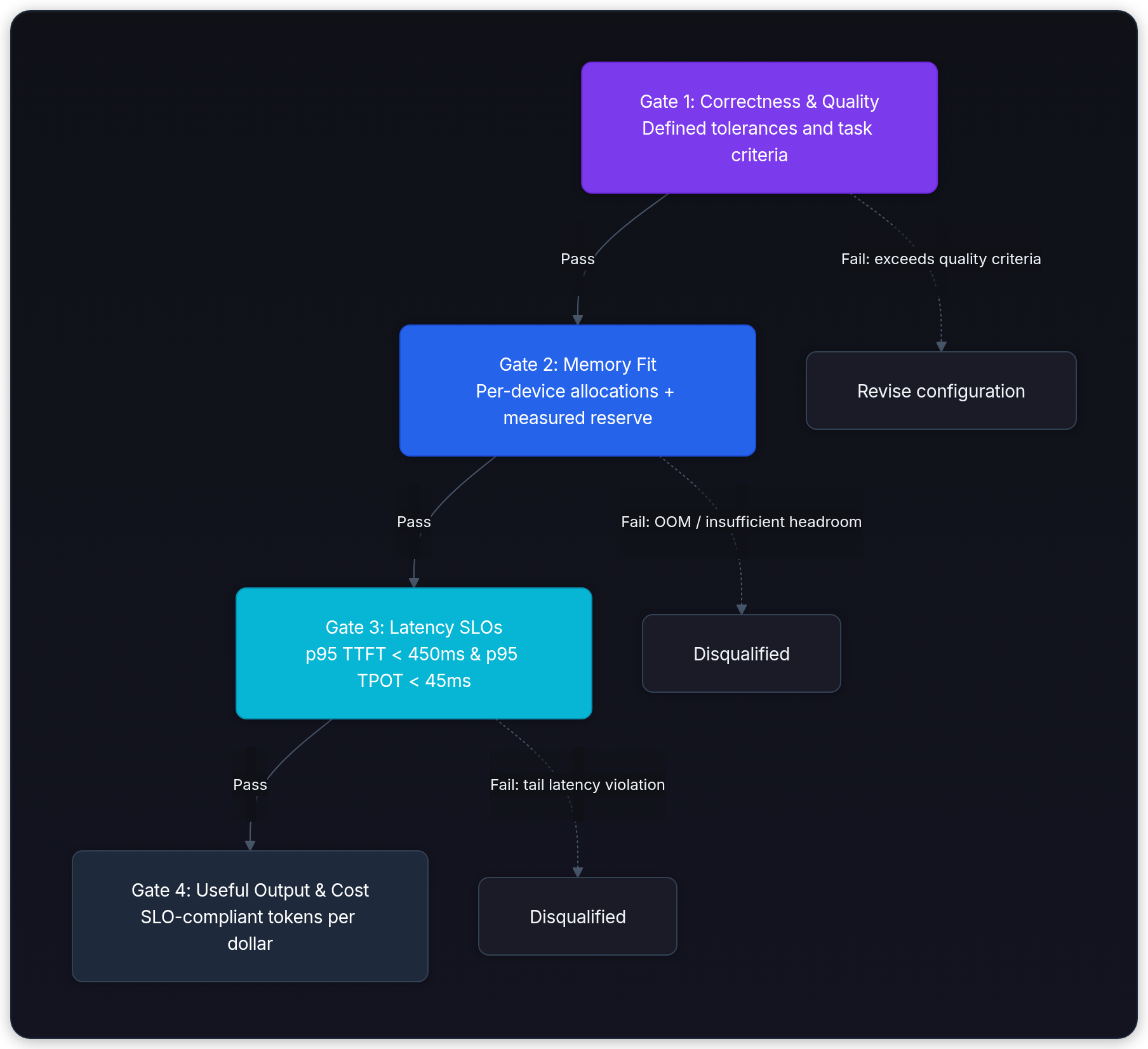
The four-gate hardware evaluation funnel

Suppose the assistant must meet p95 TTFT below 450 ms and p95 TPOT below 45 ms for eight 4,096-token prompts. Those thresholds are exercise inputs, not published accelerator results.

For this exercise, evaluate correctness, fit, and latency before ranking cost. Real investigations can revisit earlier checks as a configuration changes. The thresholds belong to this application; they aren't universal accelerator requirements.

Gate 1: Correctness and numerical precision

Evaluate whether the candidate runs the model accurately across supported precisions:

• Dtype mechanics: Establish a BF16 or other suitable reference. Evaluate reduced formats only where the exact device, kernel, and model configuration support them. FP8 variants and block-scaled formats such as MXFP4 and NVFP4 have different encoding and scaling contracts.
• Tolerance verification: Check layer outputs using predefined absolute and relative tolerances. Inspect nonfinite values and numerical extremes, then measure the application's tasks with enough examples to assess variation. A single benchmark score doesn't establish equal quality.
• Decision: Accept the configuration only if it meets the declared numerical and task-quality criteria. Rounding differences and bounded quantization error are expected; bit-for-bit equality or zero score change isn't a general requirement. Investigate NaN/Inf values in outputs expected to be finite.

Gate 2: Memory fit and residency

Calculate the full memory ledger before launching serving benchmarks:

• For the illustrative 8B BF16 model, raw weights consume about 16 decimal GB. KV size also needs the actual layers, KV heads, head dimensions, dtypes, and context allocation. Hybrid attention and recurrent-state layouts need their own terms.
• Build the ledger per device. Include graph captures, padding, communication buffers, runtime workspace, and any preallocated KV pool. Live histories occupy that pool; don't add them again as separate physical allocations.
• Measure peak allocations over expected shapes and bursts, choose a reserve from that evidence, and test admission limits. A fixed 10% or 15% margin doesn't guarantee against OOM. On Apple silicon, include the operating system and other processes sharing memory.
• Decision: The target concurrency must fit under the measured allocation and admission policy. If offload or preemption is part of the design, include its effects in the latency test.

Gate 3: Latency SLOs under production concurrency

Measure response times under the target prompt arrival distribution:

• TTFT (Time to First Token): Includes queueing, prefill, first-token production, and transport within the chosen boundary.
• TPOT (Time per Output Token): Reflects subsequent generation, batching, communication, and delivery. Also inspect individual inter-token gaps; a request average can hide a pause.
• Decision: Disqualify any candidate that fails either p95 TTFT (<450 ms) or p95 TPOT (<45 ms), regardless of its peak batch throughput.

Gate 4: Goodput and cost-efficiency

Only configurations that clear Gates 1, 2, and 3 compete on efficiency:

• Goodput: Define the eligible work. One useful metric counts output tokens from successful requests that meet both per-request latency limits, divided by the full observation interval. Report failed requests separately, including retries and cancellations.
• Cost calculation: Divide eligible tokens by cost over the same interval. Use cloud charges or an amortized owned-hardware model with energy and operating costs; don't add the provider's capital cost to a rental price already paying for it. Include idle capacity and relevant CPU, network, and storage costs.
• Decision: Rank configurations that pass this application's criteria by useful tokens per dollar, with uncertainty and workload conditions attached.

Two marginal p95 checks don't tell you whether the same requests passed both limits. Here is a twenty-request trace with one slow-first-token request and a different slow-generation request. Rates and limits are exercise values. Use nearest-rank percentiles explicitly.

from math import ceil

requests = [(500 if i == 0 else 100, 60 if i == 1 else 20, 100)
            for i in range(20)]  # TTFT ms, average TPOT ms, output tokens

def p95(values):
    ordered = sorted(values)
    return ordered[ceil(0.95 * len(ordered)) - 1]

first_ok = sum(first < 450 for first, _, _ in requests)
generation_ok = sum(gap < 45 for _, gap, _ in requests)
joint = [(first, gap, tokens) for first, gap, tokens in requests
         if first < 450 and gap < 45]
print(f"p95 TTFT={p95([r[0] for r in requests])} ms, "
      f"p95 TPOT={p95([r[1] for r in requests])} ms")
print(f"individual pass rates: {first_ok / 20:.0%}, {generation_ok / 20:.0%}")
print(f"joint pass rate: {len(joint) / 20:.0%}")
print(f"eligible output over 10 s: {sum(r[2] for r in joint) / 10:.0f} token/s")

p95 TTFT=100 ms, p95 TPOT=20 ms
individual pass rates: 95%, 95%
joint pass rate: 90%
eligible output over 10 s: 180 token/s

This small trace demonstrates metric definitions, not a reliable production tail estimate. Each marginal p95 passes, while only 90% of requests pass both limits. If the product requires 95% joint compliance, this candidate fails that additional gate.

The field guide leaves one unresolved problem: each diagnosis above depends on trustworthy timing, traces, counters, and output comparisons. The next lesson turns those words into a repeatable benchmark and correctness workflow.