Privacy-Preserving Machine Learning

Imagine a support copilot in its final security review. An analyst prompts it with "Incident 4092: Customer reported recurring billing error on...". It completes the sentence with a customer's address and a private medical note.

This is a hypothetical incident, and the output alone doesn't identify its cause. Did a retrieval tool fetch an unauthorized ticket? Was the note already in the prompt? Was it published elsewhere, or memorized during training? Trace the data path before diagnosing training leakage.

Suppose the investigation confirms training-data extraction. Removing names can reduce exposure, but it doesn't establish a guarantee about the remaining text. Addresses, unusual phrases, and combinations of facts can still identify someone. Memorization depends on the data, repetition, training, and attack; an unusual sentence isn't automatically memorized.^{[1]Reference 1Extracting Training Data from Large Language Modelshttps://arxiv.org/abs/2012.07805}

Differential privacy asks a different question: how much could the distribution of released outputs change if one declared protected contribution changed? The contribution might be a row or a person's entire history. The choice determines the promise.^{[2]Reference 2Calibrating Noise to Sensitivity in Private Data Analysis.https://people.csail.mit.edu/asmith/PS/sensitivity-tcc-final.pdf[3]Reference 3The Algorithmic Foundations of Differential Privacy.https://www.microsoft.com/en-us/research/publication/algorithmic-foundations-differential-privacy/}

We'll choose that unit, verify clipping on small vectors, compute a training budget with a real accountant, and decide which releases the budget covers.

Our training setup uses the central privacy model: a trusted service sees raw records; the released model must meet the privacy contract. Queries using that model and no additional private data inherit its guarantee. Raw databases, prompts, retrieval tools, and internal logs need their own controls. DP bounds the effect of protected participation; it doesn't prevent every sensitive inference or erase facts someone already knows.

What an attack test can tell you

Regex redaction masks recognized strings. Privacy evaluation also asks whether the remaining text or model behavior reveals information. Three useful attack families are:

1. Memorization and extraction: Probe for verbatim training text, for example by supplying prefixes. Controlled experiments can insert synthetic secrets, called canaries, at different repetition counts and test their recoverability. Published language-model work extracted sequences present in just one training document; that is a demonstrated possibility, not a rule for every rare sequence.^{[1]Reference 1Extracting Training Data from Large Language Modelshttps://arxiv.org/abs/2012.07805}
2. Membership inference (MIA): Test whether a candidate document belonged to training.^{[4]Reference 4Membership Inference Attacks against Machine Learning Modelshttps://arxiv.org/abs/1610.05820} Low loss can be a signal, but familiar or easy non-member text can also have low loss. Reference-model scores and compressed text length can help calibrate difficulty. The reference needn't have a disjoint training set. These scores support an attack decision; they don't reveal membership with certainty.^{[1]Reference 1Extracting Training Data from Large Language Modelshttps://arxiv.org/abs/2012.07805}
3. Attribute inference or reconstruction: Combine partial information with model outputs to guess sensitive fields. Some success comes from population correlations rather than one person's contribution. DP permits learning population patterns, so it doesn't promise to make every such guess impossible.^{[3]Reference 3The Algorithmic Foundations of Differential Privacy.https://www.microsoft.com/en-us/research/publication/algorithmic-foundations-differential-privacy/}

A weak attack can miss real leakage. A successful, statistically sound attack can supply evidence against a claimed guarantee. Neither result substitutes for checking the mechanism and its assumptions. DP's inequality holds for every output event, including events chosen by an adversary with background knowledge.

Start with the unit you promise to protect

Before configuring an epsilon or tuning noise scales, write one concrete contract: "one protected unit is ___." Two datasets are neighbors when they differ by that single protected unit.

In enterprise support data, that unit might be one row, one conversation ticket, or one customer account.

Suppose Alice submitted twelve support messages across three tickets. A row-level guarantee bounds what happens when one message is removed. A user-level guarantee bounds what happens when all twelve messages disappear simultaneously. That's the exact same corpus under two completely different neighboring relations, yielding two radically different privacy promises.

The definition also depends on the adjacency convention:

• Add/remove adjacency: One protected unit is added or removed. Removing a user can remove many rows.
• Replace-one adjacency: One unit's complete value is replaced, keeping the number of units fixed.

Treat the dataset as a multiset of protected units, preserving repeated contributions. For a sum of vectors whose individual norms are at most $C$, add/remove sensitivity is at most $C$; replace-one sensitivity is at most $2C$. Both bounds can be attained in one dimension. This factor of two is about this clipped sum, not a universal law for every query.

For every measurable output event $S$, a randomized mechanism $M$ satisfies $(\varepsilon,\delta)$-differential privacy if:^{[3]Reference 3The Algorithmic Foundations of Differential Privacy.https://www.microsoft.com/en-us/research/publication/algorithmic-foundations-differential-privacy/}

The probabilities reflect the internal randomness of mechanism $M$, not randomness in picking the training dataset. The condition must hold in both directions ($D$ to $D'$ and $D'$ to $D$) for every neighboring pair and every measurable output event $S$.

With $\delta=0$, epsilon bounds the ratio of event probabilities by $e^\varepsilon$ in both directions. At $\varepsilon=0.5$, an event with probability $0.001$ on one neighbor has probability at most about $0.00165$ on the other. These are probabilities, not odds. At $\varepsilon=8$, the multiplier is about $2{,}981$, a much weaker limit.

With $\delta>0$, the bound includes additive slack: that example becomes $0.00165+\delta$. Delta isn't generally a fixed fraction of people exposed, or a universal probability that a per-run guarantee “switches off.” Approximate DP permits density ratios to exceed $e^\varepsilon$ on some outputs while bounding event probabilities.

Why insist on a small delta? A mechanism that publishes its entire dataset with probability $\delta$ and otherwise returns a constant satisfies $(0,\delta)$-DP. Also, publishing one uniformly selected raw unit illustrates why delta around $1/N$ can be dangerous. Here $N$ counts protected units, not necessarily rows.

Choosing delta much below $1/N$ is common guidance, not part of the definition. NIST discusses more conservative targets such as $1/N^2$ or $1/(N\log N)$ and calls for justifying unusually large values. Choose and document it for the population and risk; don't copy $10^{-5}$ as a universal safe default.^{[5]Reference 5Guidelines for Evaluating Differential Privacy Guaranteeshttps://nvlpubs.nist.gov/nistpubs/SpecialPublications/NIST.SP.800-226.pdf} Setting $\delta=0$ gives pure DP.

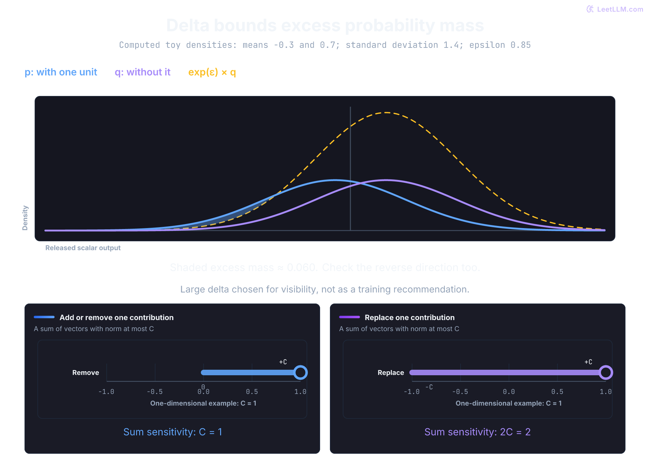
For densities $p$ and $q$, the largest excess over all events is $\int\max(p(s)-e^\varepsilon q(s),0)\,ds$. Approximate DP bounds this quantity by delta and also requires the reverse-direction bound. Gaussian densities with different means have unbounded likelihood ratios in the tails; overlapping curves alone don't prove DP.^{[6]Reference 6Fine-Tuning Large Language Models with User-Level Differential Privacyhttps://arxiv.org/abs/2407.07737}

Consider a toy mechanism you can evaluate by hand. A support customer answers a sensitive yes/no question truthfully with probability $0.75$ and reports the opposite answer with probability $0.25$:

The largest probability ratio for either output, in either direction, is $0.75/0.25=3$. Thus $\varepsilon=\ln 3$ and $\delta=0$. Every event is a subset of these two outputs, so checking both singleton outputs suffices here. Adding this randomness on the client, before the collector sees the response, gives local DP.^{[3]Reference 3The Algorithmic Foundations of Differential Privacy.https://www.microsoft.com/en-us/research/publication/algorithmic-foundations-differential-privacy/}

import math

yes_input = {"Yes": 0.75, "No": 0.25}
no_input = {"Yes": 0.25, "No": 0.75}
ratios = [
    ratio
    for output in yes_input
    for ratio in (
        yes_input[output] / no_input[output],
        no_input[output] / yes_input[output],
    )
]
print(f"largest probability ratio: {max(ratios):.1f}")
print(f"epsilon: {math.log(max(ratios)):.3f}, delta: 0")

largest probability ratio: 3.0
epsilon: 1.099, delta: 0

This example verifies probabilities; it doesn't collect private responses. Central DP training uses a trusted service instead, and needs a mechanism for the entire released training result.

Mechanisms and sensitivity scaling

Differential privacy adds noise proportional to the query's global sensitivity. For any function $f$ mapping a dataset to a vector space, sensitivity measures the maximum change between any two neighboring datasets $D$ and $D'$:

Two foundational mechanisms inject this noise:

The Laplace mechanism adds independent noise drawn from $\text{Lap}(\Delta_1 f / \varepsilon)$ to each coordinate. It guarantees pure $(\varepsilon, 0)$-differential privacy. For scalar counts or low-dimensional database queries, Laplace noise is simple and effective.

For a $d$-dimensional vector, $\|v\|_1\le\sqrt d\,\|v\|_2$. An $L_2$ sensitivity bound can therefore imply a larger $L_1$ bound. Coordinate-wise Laplace calibration may be costly in this setting; it doesn't universally make neural-network optimization fail.

The Gaussian mechanism adds $\mathcal{N}(0,s^2 I)$. One classical sufficient calibration, for $0<\varepsilon<1$ and $0<\delta<1$, is:^{[3]Reference 3The Algorithmic Foundations of Differential Privacy.https://www.microsoft.com/en-us/research/publication/algorithmic-foundations-differential-privacy/}

This is sufficient, not the tightest calibration, and its stated epsilon range matters. Analytical Gaussian calibration uses the Gaussian cumulative distribution function and avoids limitations of this classical bound.^{[7]Reference 7Improving the Gaussian Mechanism for Differential Privacy: Analytical Calibration and Optimal Denoisinghttps://proceedings.mlr.press/v80/balle18a.html} Gaussian noise and its composition analysis are standard ingredients in DP-SGD. They don't establish a universal utility ranking over all mechanisms.

We'll use $s$ for an actual standard deviation. In DP-SGD below, $\sigma$ is a dimensionless noise multiplier, and the standard deviation on the clipped sum is $\sigma C$.

Differentially private stochastic gradient descent

Ordinary SGD averages a mini-batch's gradients and updates the parameters. Without a contribution bound, one gradient can change that average substantially. A large gradient isn't itself evidence of private text or memorization.

Differentially private stochastic gradient descent (DP-SGD) combines bounded contributions with calibrated randomness and accounting.^{[8]Reference 8Deep Learning with Differential Privacyhttps://arxiv.org/abs/1607.00133}

Consider a record-level, add/remove DP-SGD variant. Its Poisson sampler independently includes each present record with public probability $q$. Let $L$ be a fixed public normalizer, unchanged between neighbors; commonly $L=qN$ for a public reference population size $N$. Using a private, changing record count as a published normalizer needs separate analysis.

Each step $t$ has five phases:

1. Poisson subsampling: Include each record independently with probability $q$, forming a random-size batch $B_t$. Other samplers require accounting that matches them.
2. Per-sample gradients: Obtain each contribution $g_i(\theta_t)=\nabla_\theta\mathcal L(x_i,\theta_t)$ and its clipping factor before reduction. Efficient methods such as ghost clipping can do this without materializing every full per-example gradient tensor.^{[9]Reference 9Large Language Models Can Be Strong Differentially Private Learnershttps://arxiv.org/abs/2110.05679}
3. Per-sample clipping: Enforce an $L_2$ norm threshold $C > 0$ on each vector: $$\bar{g}_i(\theta_t) = g_i(\theta_t) \cdot \min\left(1, \frac{C}{\|g_i(\theta_t)\|_2}\right)$$ Leave a zero vector unchanged, avoiding division by zero. Other vectors retain their direction; norms above $C$ shrink to $C$.
4. Summation and Gaussian noise injection: Sum the clipped vectors and add calibrated Gaussian noise scaled to sensitivity $C$: $$\widetilde{g}_t = \sum_{i \in B_t} \bar{g}_i(\theta_t) + \mathcal{N}\left(0, \sigma^2 C^2 I\right)$$ Conditional on the previous accounted state, adding or removing one sampled contribution changes the clipped sum by at most $C$. The multiplier, sampling, and number of steps determine the composed privacy guarantee.
5. Descent step: Divide the noisy aggregate by target batch size $L$ and update parameters: $$\theta_{t+1} = \theta_t - \eta_t \frac{\widetilde{g}_t}{L}$$

A frequent bug in custom implementations is clipping the batch average after aggregation: clip(mean(gradients), C). This bounds the final update vector's length to $C$, but neighboring dataset averages can still point in opposite directions, creating a worst-case difference of $2C$ between outputs. Clipping must occur per sample before aggregation to establish sensitivity $C$ for the batch sum.

Verify the geometry on three vectors. This deterministic example is not a DP release: it adds no noise. Keep full precision during aggregation and round only the display; rounding a clipped vector first can push its norm above $C$.

import math

def clip_vector_l2(vector: list[float], bound: float) -> list[float]:
    if type(bound) not in (int, float) or not math.isfinite(bound) or bound <= 0:
        raise ValueError("bound must be positive and finite")
    if not vector or any(
        type(x) not in (int, float) or not math.isfinite(x) for x in vector
    ):
        raise ValueError("vector must contain finite numeric coordinates")
    norm = math.hypot(*vector)
    if not math.isfinite(norm):
        raise ValueError("norm exceeds this toy implementation's numeric range")
    if norm == 0.0 or norm <= bound:
        return list(vector)
    scale = bound / norm
    return [x * scale for x in vector]

sample_gradients = [
    [0.4, 0.3],    # norm = 0.5 <= 1.0 (unclipped)
    [3.0, 4.0],    # norm = 5.0 > 1.0 (scaled by 1.0 / 5.0 = 0.2)
    [0.6, 0.8],    # norm = 1.0 == 1.0 (unclipped)
]
clip_bound = 1.0
clipped = [clip_vector_l2(g, clip_bound) for g in sample_gradients]

print(f"sample gradients: {sample_gradients}")
print(f"clipped gradients: {[[round(x, 4) for x in g] for g in clipped]}")

sum_g = [sum(dim) for dim in zip(*clipped)]
print(f"clipped sum before noise: [{sum_g[0]:.2f}, {sum_g[1]:.2f}]")

sample gradients: [[0.4, 0.3], [3.0, 4.0], [0.6, 0.8]]
clipped gradients: [[0.4, 0.3], [0.6, 0.8], [0.6, 0.8]]
clipped sum before noise: [1.60, 1.90]

The outlier [3.0, 4.0] scales to [0.6, 0.8], with norm $1$. Contrast [1.0, 3.0]: rounding its clipped coordinates to [0.3162, 0.9487] gives a norm slightly above $1$. The displayed decimals aren't the vector you should aggregate. Production DP needs a vetted implementation, including numerical behavior.

Now consider what happens when Alice contributes multiple messages. If Alice wrote two tickets with gradients $0.5$ and $5.0$, example-level clipping bounds each message to $1.0$, leaving Alice with a combined influence of $1.5$. It doesn't give Alice a single $C$ bound. A known limit of $k$ clipped records permits a $kC$ sum bound; unlimited records don't.

One user-level construction groups records, builds a vector per user, and clips that vector.^{[6]Reference 6Fine-Tuning Large Language Models with User-Level Differential Privacyhttps://arxiv.org/abs/2407.07737} It can use a sum or an average defined by the mechanism. Other constructions use per-example clipping plus bounded records per user and user-level analysis. Simply renaming a row-level accountant doesn't protect users.

Here's the sum-then-user-clip geometry, again without noise. Alice's two tickets and Bao's one ticket use a fixed public normalizer of two:

import math

def clip_scalar(gradient: float, bound: float) -> float:
    if type(bound) not in (int, float) or not math.isfinite(bound) or bound <= 0:
        raise ValueError("bound must be positive and finite")
    if type(gradient) not in (int, float) or not math.isfinite(gradient):
        raise ValueError("gradient must be finite")
    return max(-bound, min(gradient, bound))

user_gradients = {"Alice": [0.5, 5.0], "Bao": [0.25]}
clip_bound = 1.0

for user, gradients in user_gradients.items():
    row_clipped_sum = sum(clip_scalar(value, clip_bound) for value in gradients)
    user_clipped = clip_scalar(sum(gradients), clip_bound)
    print(f"{user}: row-clipped sum={row_clipped_sum:.2f}, user-clipped={user_clipped:.2f}")

normalizer = 2  # Public and unchanged across neighboring datasets.
user_contributions = {
    user: clip_scalar(sum(values), clip_bound)
    for user, values in user_gradients.items()
}
with_alice = sum(user_contributions.values()) / normalizer
without_alice = user_contributions["Bao"] / normalizer
print(f"with Alice, before noise: {with_alice:.3f}")
print(f"without Alice, before noise: {without_alice:.3f}")
print(f"change from removing Alice: {with_alice - without_alice:.3f}")
assert abs(with_alice - without_alice) <= clip_bound / normalizer

Alice: row-clipped sum=1.50, user-clipped=1.00
Bao: row-clipped sum=0.25, user-clipped=0.25
with Alice, before noise: 0.625
without Alice, before noise: 0.125
change from removing Alice: 0.500

Removing Alice changes the normalized sum by $C/2=0.5$. The unnormalized user contribution is bounded by $C$ regardless of her ticket count. A full user-level training guarantee must also match user sampling, noise calibration, and composition.

Account for every exposed release

Clipping bounds sensitivity for one training step. Training an LLM takes thousands of steps. A privacy accountant tracks how privacy loss accumulates over the full optimization run ^{[10]Reference 10Compute DP-SGD Privacyhttps://opacus.ai/api/compute_dp_sgd_privacy.html}.

Basic composition adds valid conditional step budgets: $(\sum_t\varepsilon_t,\sum_t\delta_t)$. For example, $5{,}000$ steps each charged epsilon $0.1$ give a conservative epsilon $500$. This bound can be very loose.

The moments accountant and Rényi differential privacy (RDP) exploit more information about the mechanism.^{[8]Reference 8Deep Learning with Differential Privacyhttps://arxiv.org/abs/1607.00133[11]Reference 11Rényi Differential Privacyhttps://arxiv.org/abs/1702.07476} For neighboring output densities $p$ and $p'$ and order $\alpha>1$, Rényi divergence is:

An RDP bound $\varepsilon_t^{\mathrm{RDP}}(\alpha)$ must hold for all neighbors, in both directions, conditional on earlier released states. Such bounds add:

For a chosen $0<\delta<1$, a valid conservative conversion is:^{[11]Reference 11Rényi Differential Privacyhttps://arxiv.org/abs/1702.07476}

Here $\mathcal A$ is the set of analyzed orders. Accountants can use tighter conversions. For an unsampled Gaussian mechanism with sensitivity $C$ and standard deviation $\sigma C$, the per-step RDP bound is $\alpha/(2\sigma^2)$. Subsampling changes the analysis; don't insert a rough $q^2$ multiplier and treat it as a certified budget.

Subsampling amplification exploits the random inclusion of a protected unit when the sample identity isn't released. The observer sees an output distribution that mixes inclusion and non-inclusion cases. They can still infer something about participation. A Poisson accountant must match the actual sampler, adjacency, protected unit, and clipping mechanism.

Compute a concrete budget with Opacus's RDPAccountant.^{[12]Reference 12RDPAccountanthttps://opacus.ai/api/accounting/rdp.html} This example pins version 1.6.0, checked September 21, 2026. It charges 300 or 600 Poisson-sampled Gaussian steps at $q=0.01$, multiplier $\sigma=1$, and $\delta=10^{-5}$:

from opacus.accountants import RDPAccountant

for steps in [300, 600]:
    accountant = RDPAccountant()
    for _ in range(steps):
        accountant.step(noise_multiplier=1.0, sample_rate=0.01)
    epsilon = accountant.get_epsilon(delta=1e-5)
    print(f"steps={steps}, epsilon={epsilon:.3f}, delta=1e-5")

steps=300, epsilon=1.451, delta=1e-5
steps=600, epsilon=1.748, delta=1e-5

For these settings, doubling steps increases the reported bound from $1.451$ to $1.748$. That isn't a universal square-root law or evidence of model quality. The accountant computes a bound from supplied parameters; it doesn't inspect your optimizer and prove that your training code satisfies them.

What about serving ten million queries? The post-processing theorem says that computations using the accounted DP output and no additional unprotected private data preserve its training-data guarantee.^{[3]Reference 3The Algorithmic Foundations of Differential Privacy.https://www.microsoft.com/en-us/research/publication/algorithmic-foundations-differential-privacy/} Query count alone adds no training epsilon. This doesn't protect the contents of new private prompts or authorize retrieval from a raw ticket database.

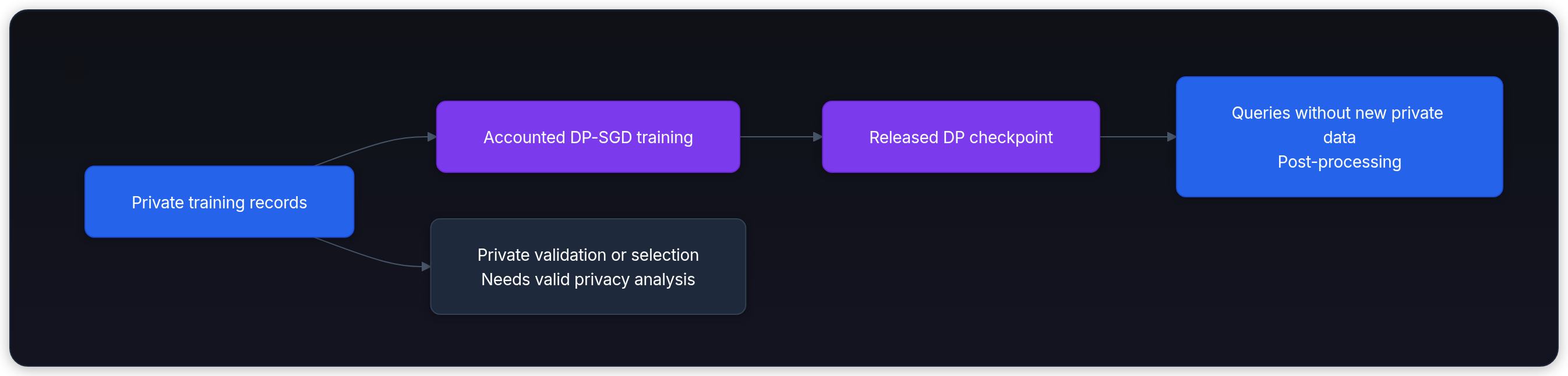
Private validation needs care even if you don't publish its score: selecting a released model using raw private scores can leak information through the choice. Use public validation or a valid private evaluation/selection mechanism with accounting. Publishing raw gradients or unprotected diagnostics may have no useful finite budget; don't just charge them an arbitrary epsilon.

Checkpoints aren't automatically independent new charges. If the accountant already bounds the joint transcript of all noisy training updates, releasing multiple checkpoints derived only from that transcript is post-processing of the accounted run. Separate training runs on overlapping users generally need composition. Disjoint protected populations can permit parallel composition. Record which analysis covers each artifact so you neither omit exposure nor charge the same transcript twice.

For a simple exercise, suppose two completed runs and a candidate reuse protected users. Each has a verified guarantee for the same adjacency, conditional on earlier releases. Add their budgets conservatively and compare them with a local cap:

from decimal import Decimal, localcontext

def compose_release(released, candidate, epsilon_cap, delta_cap):
    def check_budget(pair):
        if not isinstance(pair, (tuple, list)) or len(pair) != 2:
            raise ValueError("budget must be an epsilon/delta pair")
        epsilon, delta = pair
        if any(type(value) is not Decimal or not value.is_finite() for value in pair):
            raise ValueError("budget values must be finite Decimals")
        if epsilon < 0 or not 0 <= delta < 1:
            raise ValueError("budget requires epsilon >= 0 and 0 <= delta < 1")
        return epsilon, delta

    check_budget((epsilon_cap, delta_cap))
    budgets = [check_budget(pair) for pair in [*released, candidate]]
    values = [value for pair in budgets for value in pair]
    lowest_exponent = min(value.as_tuple().exponent for value in values)
    highest_digit = max(value.adjusted() for value in values)
    with localcontext() as context:
        context.prec = max(28, highest_digit - lowest_exponent + len(str(len(budgets))) + 2)
        total_epsilon = sum((eps for eps, _ in budgets), Decimal("0"))
        total_delta = sum((delta for _, delta in budgets), Decimal("0"))
    allowed = total_epsilon <= epsilon_cap and total_delta <= delta_cap
    return total_epsilon, total_delta, allowed

released = [
    (Decimal("1.2"), Decimal("0.000001")),
    (Decimal("1.1"), Decimal("0.000001")),
]
candidate = (Decimal("0.9"), Decimal("0.000001"))
proposed_epsilon, proposed_delta, allowed = compose_release(
    released, candidate, Decimal("3.0"), Decimal("0.000003")
)

print(f"candidate total: epsilon={proposed_epsilon:.1f}, delta={proposed_delta:.6f}")
print(f"release allowed: {allowed}")
assert not allowed

candidate total: epsilon=3.2, delta=0.000003
release allowed: False

The calculation rejects the candidate because $3.2>3.0$. Finite Decimal inputs avoid binary floating-point surprises, and the local precision accommodates the sum rather than silently rounding a tiny excess down to the cap. Negative or non-finite entries are rejected. The function doesn't authenticate receipts, validate training assumptions, or control deployment. Those remain host responsibilities.

The privacy-utility trade-off in modern LLMs

Noise geometry helps explain a cost of private training, but it doesn't predict accuracy on its own.

For sum noise $Z\sim\mathcal N(0,\sigma^2C^2I_d)$ over $d$ trainable coordinates, the root mean square (RMS) norm is exactly:

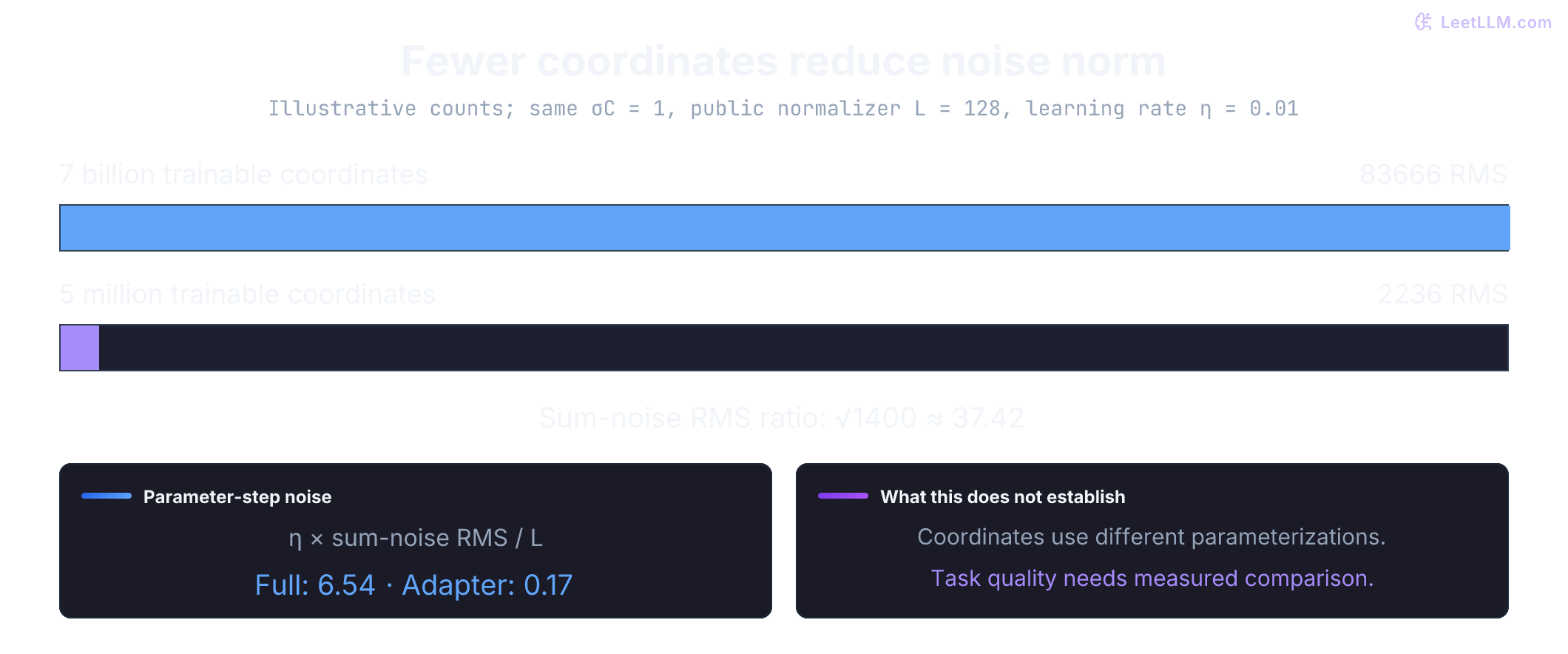
The mean norm is close to this for large $d$, but a particular draw isn't guaranteed to exceed a threshold. Crucially, DP-SGD adds this noise to the sum, then divides by $L$ and multiplies by learning rate $\eta$. The RMS norm of the resulting parameter-step noise is $\eta\sigma C\sqrt d/L$.

Actual gradient signal depends on the task, representations, clipping, and optimization. Published work shows that pretrained representations, objectives, and hyperparameters can make full private fine-tuning effective. Batch size is a tuning and accounting choice, not a universal convergence threshold. Parameter-efficient methods need comparison against a well-tuned full-fine-tuning baseline.^{[9]Reference 9Large Language Models Can Be Strong Differentially Private Learnershttps://arxiv.org/abs/2110.05679}

DP-LoRA combines a LoRA parameterization with private training. LoRA freezes base weights and learns low-rank updates:^{[13]Reference 13LoRA: Low-Rank Adaptation of Large Language Models.https://arxiv.org/abs/2106.09685}

For a linear layer acting on column vectors, let $W_0\in\mathbb R^{d_{\mathrm{out}}\times d_{\mathrm{in}}}$. Its frozen weight receives this trainable update:

For one adapted matrix, the trainable count is $r(d_{\mathrm{in}}+d_{\mathrm{out}})$ instead of $d_{\mathrm{in}}d_{\mathrm{out}}$. At rank $8$, a $4096\times4096$ matrix uses $65{,}536$ adapter parameters, about $0.39\%$ of that matrix's original count. The whole-model fraction depends on which layers are adapted and which other parameters remain trainable.

If only adapters are trained, clip and perturb their protected-unit contributions. Consider illustrative counts of $7$ billion full-model coordinates and $5$ million adapter coordinates with the same $\sigma C$, $L$, and $\eta$. The sum-noise RMS ratio is $\sqrt{7\times10^9/(5\times10^6)}\approx37.42$. Compute both the sum and step noise:

import math

sigma_c = 1.0
normalizer = 128
learning_rate = 0.01
full_sum_rms = sigma_c * math.sqrt(7_000_000_000)
adapter_sum_rms = sigma_c * math.sqrt(5_000_000)

print(f"full sum-noise RMS: {full_sum_rms:.2f}")
print(f"adapter sum-noise RMS: {adapter_sum_rms:.2f}")
print(f"RMS ratio: {full_sum_rms / adapter_sum_rms:.2f}")
print(f"full step-noise RMS: {learning_rate * full_sum_rms / normalizer:.2f}")
print(f"adapter step-noise RMS: {learning_rate * adapter_sum_rms / normalizer:.2f}")

full sum-noise RMS: 83666.00
adapter sum-noise RMS: 2236.07
RMS ratio: 37.42
full step-noise RMS: 6.54
adapter step-noise RMS: 0.17

This is coordinate-space arithmetic, not a benchmark. Adapter coordinates and full-weight coordinates describe different parameterizations; equal coordinate norms needn't imply equal changes to model outputs. Fewer coordinates don't automatically give better task accuracy, better gradient signal-to-noise ratio, or a stronger privacy budget.

Before claiming protection, inspect the base model too:

1. Existing information: If a base was pretrained non-privately, private fine-tuning doesn't retroactively protect that pretraining or erase memorized text.
2. Incremental protection: The fine-tuning proof normally holds the base and other unaccounted inputs fixed across neighbors. It bounds the change caused by protected fine-tuning contributions. It doesn't guarantee zero extraction: the base, background knowledge, and population correlations may already reveal a fact.
3. Overlapping private users: If removing a protected user should also change a privately pretrained base, holding that base fixed doesn't prove privacy for the person's entire participation. Include the base's exposure in an appropriate end-to-end analysis.

For the support copilot, require a release record naming the protected unit, adjacency, sampler, clipping, noise multiplier, step count, delta, accountant version, and covered artifacts. Evaluate usefulness and extraction separately. Then inspect retrieval permissions and prompt/log handling. A correct training guarantee addresses one important data path; the assistant's whole privacy story needs all of them.