Probabilistic Generative Models

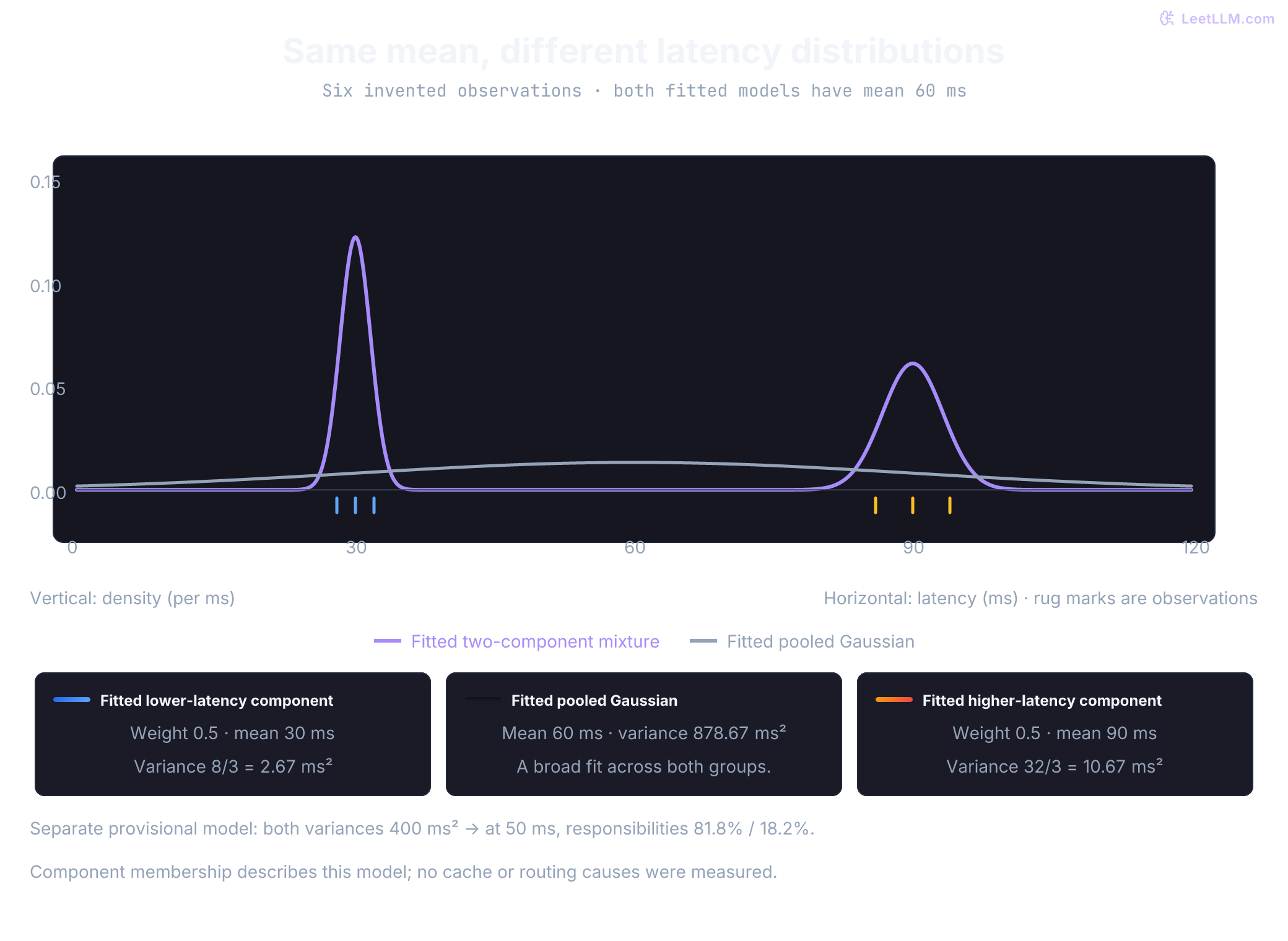
Imagine a dashboard built from six request latencies: [28, 30, 32, 86, 90, 94] milliseconds. Its mean is 60 ms, yet no measured request took 60 ms. Would you plan capacity around that average, or ask why the observations form two groups?

These are invented measurements, and we haven't recorded cache status, query plans, or routing. A single fitted Gaussian has its highest density at 60 ms and spreads broadly enough to cover both groups. A Gaussian mixture model can instead fit separate peaks and assign fractional membership. Neither fit proves that the groups correspond to two infrastructure causes, and six observations aren't enough to establish the population's shape.^{[1]Reference 1Pattern Recognition and Machine Learning.https://www.microsoft.com/en-us/research/publication/pattern-recognition-machine-learning/}

Generative versus discriminative modeling

Machine learning systems answer two distinct modeling questions depending on whether they estimate conditional or joint distributions.

In the statistical classification distinction, discriminative modeling learns to predict $Y$ from $X$, often through $P(Y \mid X)$ or a decision score. With labeled logs, a classifier might estimate cache-hit probability from latency and query size. A conditional probability alone doesn't specify the input distribution $P(X)$: many different input distributions can share the same $P(Y \mid X)$. Consequently, a large class probability isn't evidence that an input is typical. Confidence on corrupted inputs depends on the model; overconfidence isn't inevitable.

Generative modeling specifies a distribution from which we can sample observations. A generative classifier might model $P(X,Y)=P(Y)P(X \mid Y)$ and derive $P(Y \mid X)$ by Bayes' rule. An unlabeled density model instead models $p(X)$, possibly through hidden variables. It can score observations under its assumptions, but density isn't a guaranteed anomaly detector and a sampling story isn't automatically a causal explanation.^{[1]Reference 1Pattern Recognition and Machine Learning.https://www.microsoft.com/en-us/research/publication/pattern-recognition-machine-learning/}

The terminology also depends on the task. An LLM models a distribution over text conditioned on a prompt, so a conditional distribution can support generation. Here we'll use the classification distinction to ask a narrower question: how could a probability model describe our unlabeled latency sample?

Our hidden component index is a latent variable, an unobserved variable included in the statistical model. Some request logs do contain cache or routing labels. This example deliberately doesn't.

Latent variables and the coupled log-sum

Start with the six observed request latencies: [28, 30, 32, 86, 90, 94]. Their arithmetic mean is 60 ms, but the numbers naturally cluster into two distinct groups.

A probabilistic generative model formulates a two-stage story for each observation:

In the model, first select component $z_i = k \in \{1,\dots,K\}$ with probability $\pi_k$, where $\sum_k \pi_k=1$ and $\pi_k \ge 0$. Then sample $x_i$ from $p(x_i \mid z_i=k,\theta)=\mathcal{N}(x_i \mid \mu_k,\sigma_k^2)$ with $\sigma_k^2>0$. The weight $\pi_k$ describes component frequency, not confidence in a fitted mean.

Because the log records $X=\{x_1,\dots,x_n\}$ but not $Z=\{z_1,\dots,z_n\}$, calculate an observation's density by summing the contributions from its $K$ possible components:

Assume observations are independent and identically distributed under this model. Real traffic can violate that assumption through time, tenant, or queue dependence. Maximum likelihood estimation chooses parameters $\theta=\{\pi_k,\mu_k,\sigma_k^2\}_{k=1}^K$ to maximize the product of the observed densities. Its logarithm is:

Notice the mathematical barrier: the summation across components sits inside the logarithm.

For a single Gaussian with nonzero empirical variance, the mean and variance maximizing likelihood have simple formulas. For a general mixture, the log of a sum couples component parameters, so those single-Gaussian formulas don't solve the whole fit in one step. The objective is non-convex, and gradient-based optimization is possible too.^{[1]Reference 1Pattern Recognition and Machine Learning.https://www.microsoft.com/en-us/research/publication/pattern-recognition-machine-learning/}

Keep evaluation separate from optimization. With two Gaussian components, summing two densities and computing their posterior probabilities is easy and exact. The challenge here is fitting the parameters. Continuous latent variables replace sums with integrals; some models, including linear Gaussian models, still allow exact integration. Nonlinear neural decoders usually don't.

Soft responsibilities in Gaussian mixtures

If component labels were observed and each group had positive empirical variance, we'd fit separate Gaussian means and variances. With parameters already fixed, we'd instead calculate posterior membership using Bayes' rule.

Because we have neither, we start by evaluating provisional parameters. Consider two provisional components: a fast component at $\mu_1 = 30$ ms, a slow component at $\mu_2 = 90$ ms, equal standard deviations $\sigma_1 = \sigma_2 = 20$ ms, and equal prior weights $\pi_1 = \pi_2 = 0.5$.

Now evaluate a new request at 50 ms, between the two means. The fast Gaussian's density there is roughly 0.01210 per ms; the slow Gaussian's density is roughly 0.00270 per ms. Weighting each by 0.5 gives contributions 0.00605 and 0.00135. The equal-responsibility boundary for this model is 60 ms.

Normalizing these two numbers yields the posterior probability that component $k$ generated observation $x_i$, known as the component's responsibility $\gamma_{ik}$:^{[1]Reference 1Pattern Recognition and Machine Learning.https://www.microsoft.com/en-us/research/publication/pattern-recognition-machine-learning/}

For our 50 ms request, the fast responsibility is $0.00605 / (0.00605 + 0.00135) \approx 0.818$, and the slow responsibility is $0.00135 / 0.00740 \approx 0.182$. The next code snippet calculates these values without intermediate rounding:

from math import exp, pi, sqrt

def gaussian_density(value: float, mean: float, deviation: float) -> float:
    exponent = -((value - mean) ** 2) / (2 * deviation**2)
    return exp(exponent) / (sqrt(2 * pi) * deviation)

latency = 50.0
weighted_fast = 0.5 * gaussian_density(latency, mean=30.0, deviation=20.0)
weighted_slow = 0.5 * gaussian_density(latency, mean=90.0, deviation=20.0)
total = weighted_fast + weighted_slow

fast = weighted_fast / total
slow = weighted_slow / total
assert abs(fast + slow - 1.0) < 1e-12
print(f"fast responsibility: {fast:.3f}")
print(f"slow responsibility: {slow:.3f}")

fast responsibility: 0.818
slow responsibility: 0.182

The fast component receives greater responsibility here because its mean is closer and variances are equal. If components had unequal spreads or priors, the closer mean wouldn't automatically win.

Keep the observation, means, and spreads fixed, but suppose the fast component's prior weight is 0.1 instead of 0.5. Reuse the density function to isolate that change:

weighted_fast = 0.1 * gaussian_density(latency, mean=30.0, deviation=20.0)
weighted_slow = 0.9 * gaussian_density(latency, mean=90.0, deviation=20.0)
fast = weighted_fast / (weighted_fast + weighted_slow)
print(f"fast responsibility with prior 0.1: {fast:.3f}")
print(f"slow responsibility with prior 0.9: {1 - fast:.3f}")

fast responsibility with prior 0.1: 0.332
slow responsibility with prior 0.9: 0.668

The likelihood ratio favors the closer fast component by about 4.48 to 1, but its prior odds are 1 to 9. Multiplying them gives posterior odds about 0.498 to 1, so the slow component wins. This is the same Bayes update used in Bayesian Inference. A responsibility combines component frequency with fit to the observation; it isn't just a softened nearest-center rule.

Compare this with K-means, which assigns each point to a nearest center. With shared spherical covariance $\Sigma_k=\sigma^2 I$, responsibilities satisfy

Hold centers and positive priors fixed while $\sigma^2 \to 0$. A uniquely closest center receives responsibility approaching one. At an exact distance tie, responsibilities stay proportional to the tied components' priors; shrinking variance doesn't break the tie. The weighted mean update then approaches K-means' mean update when assignments are unique and clusters are nonempty. This limiting argument uses a shared variance; it isn't an instruction to shrink each fitted GMM variance toward zero.

The 0.818/0.182 split expresses membership under the provisional model, not measured physical uncertainty or verified cache-versus-database probabilities.

Responsibilities are discrete probabilities summing to one for each observation ($\sum_k \gamma_{ik} = 1$). In contrast, $p(x \mid \theta)$ is a continuous probability density, whose values can exceed 1.0 for narrow spreads and whose integral over an interval gives probability.

Expectation-Maximization as lower-bound ascent

We need responsibilities to learn parameters, but we need parameters to calculate responsibilities. The expectation-maximization (EM) algorithm alternates between the two. Dempster, Laird, and Rubin's classic 1977 paper formalized the general algorithm and its likelihood-improvement argument.^{[2]Reference 2Maximum Likelihood from Incomplete Data via the EM Algorithmhttps://doi.org/10.1111/j.2517-6161.1977.tb01600.x}

Introduce a probability distribution $q(Z)$ over the latent variables and an evidence lower bound (ELBO) on the log likelihood. Whether the bound is practical to calculate depends on the model and the choice of $q$. In our independent-observation GMM, both the joint model and its posterior factorize by observation, avoiding enumeration of all $K^n$ assignment vectors.

For a concave function $f$, Jensen's inequality gives $f(\mathbb{E}[Y]) \ge \mathbb{E}[f(Y)]$ when the expectations exist. To derive the bound below, take $q(Z)>0$ wherever $p(X,Z \mid \theta)>0$, so multiplying and dividing by $q$ doesn't discard part of the sum. The logarithm is concave:

Expanding that expectation defines the Evidence Lower Bound $\mathcal{L}(q, \theta)$:^{[3]Reference 3CS229 Machine Learning Notes: The EM Algorithmhttps://cs229.stanford.edu/notes2022fall/main_notes.pdf}

We can also express the relationship as an exact algebraic decomposition:

where $D_{\mathrm{KL}}(q \parallel p)$ is the Kullback-Leibler divergence measuring the divergence between our distribution $q(Z)$ and the true posterior $p(Z \mid X, \theta)$:

For finite terms, this decomposition identifies the gap exactly. KL divergence is nonnegative and is zero when $q$ equals the posterior (almost everywhere for continuous variables). Therefore $\mathcal{L}(q,\theta) \le \ell(\theta)$. A bound can be valid yet loose; a restricted or approximate $q$ needn't make the gap zero.

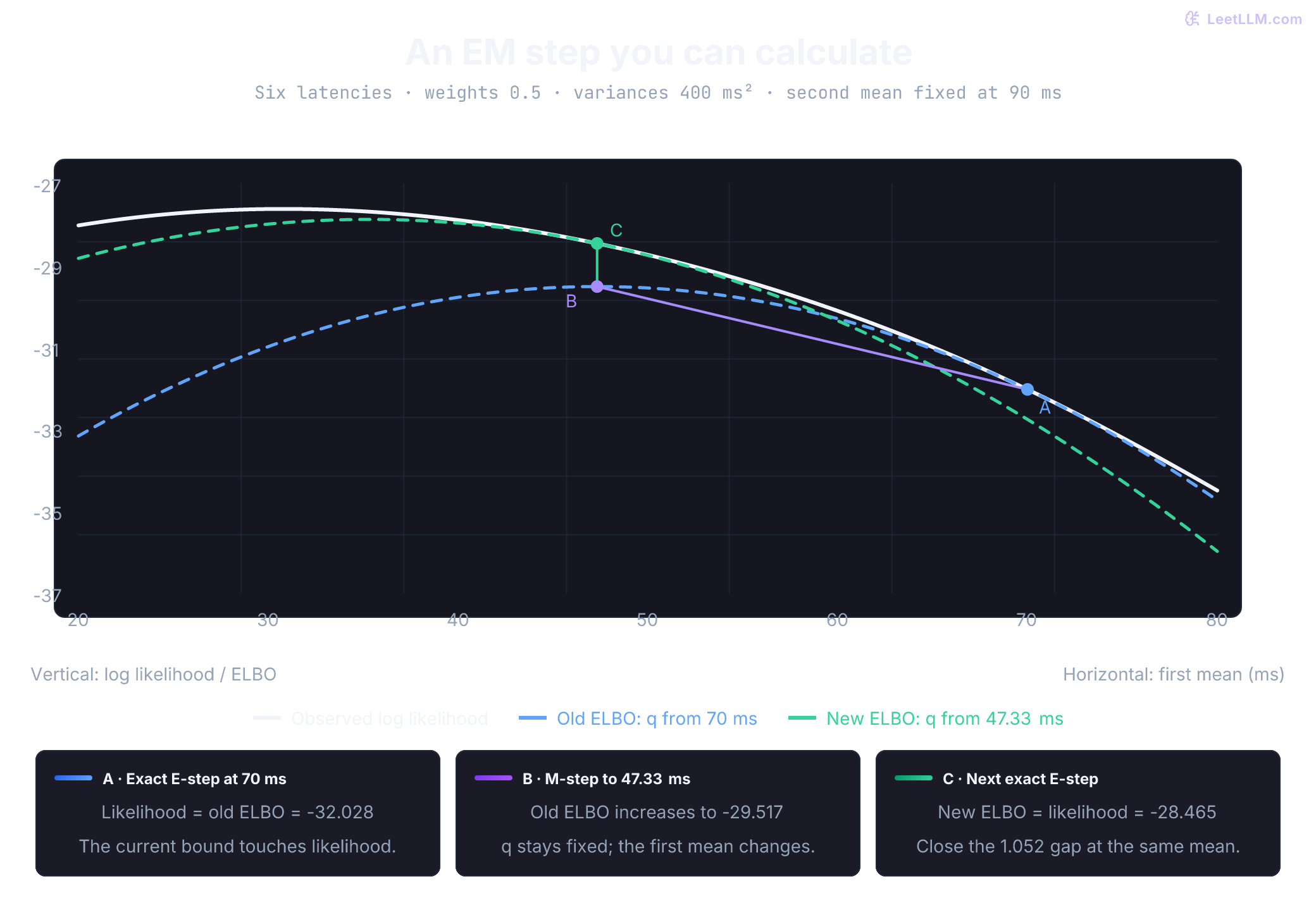
The algorithm climbs this geometry through coordinate ascent:

1. E-step: Hold $\theta^{(t)}$ fixed and compute the exact posterior $q(Z)=p(Z \mid X,\theta^{(t)})$. For the GMM, this means computing responsibilities. The gap is zero at the current parameters:

   $$\mathcal{L}(q, \theta^{(t)}) = \log p(X \mid \theta^{(t)}).$$

2. M-step: Freeze $q$ and maximize the bound over the allowed parameter space:

   $$\theta^{(t+1)} = \arg\max_\theta \mathcal{L}(q, \theta) = \arg\max_\theta \sum_{Z} q(Z) \log p(X, Z \mid \theta).$$

   The entropy $-\sum_Z q(Z)\log q(Z)$ is constant with respect to $\theta$. The remaining objective is the expected complete-data log likelihood, often called $Q$. For our GMM it separates into weighted Gaussian fits. Other models can still require numerical optimization.

3. Monotonicity guarantee: Combining both steps confirms that likelihood never decreases:^{[2]Reference 2Maximum Likelihood from Incomplete Data via the EM Algorithmhttps://doi.org/10.1111/j.2517-6161.1977.tb01600.x}

   $$\log p(X \mid \theta^{(t+1)}) \ge \mathcal{L}(q, \theta^{(t+1)}) \ge \mathcal{L}(q, \theta^{(t)}) = \log p(X \mid \theta^{(t)}).$$

Read the three comparisons from right to left: the old bound touches old likelihood, the parameter update doesn't lower that bound, and new likelihood is at least the new bound. Exact E-steps plus an M-step that merely doesn't decrease $Q$ are sufficient for this argument; that variant is generalized EM.^{[2]Reference 2Maximum Likelihood from Incomplete Data via the EM Algorithmhttps://doi.org/10.1111/j.2517-6161.1977.tb01600.x}

Monotonic means non-decreasing, not strictly improving. If likelihood is bounded above, its values converge, but that fact alone doesn't prove the parameters converge or reach a local maximum. Stationary-point results require additional regularity conditions, and unconstrained Gaussian mixtures can have unbounded likelihood. No part of the inequality certifies a global optimum.

Before fitting all parameters, reproduce the figure's restricted example. Keep means [m, 90], weights [0.5, 0.5], and both variances at 400 ms². The only free parameter is m. For each observation, q[i][k] holds its component responsibility; independence lets us sum over observations instead of all assignment vectors:

from math import exp, log, pi

observations = [28.0, 30.0, 32.0, 86.0, 90.0, 94.0]

def joint_log_scores(mean):
    return [
        [log(0.5) - 0.5 * (log(2 * pi * 400.0) + (x - mu)**2 / 400.0)
         for mu in (mean, 90.0)]
        for x in observations
    ]

def logsumexp(row):
    largest = max(row)
    return largest + log(sum(exp(value - largest) for value in row))

def likelihood(mean):
    return sum(logsumexp(row) for row in joint_log_scores(mean))

def posterior(mean):
    return [[exp(value - logsumexp(row)) for value in row]
            for row in joint_log_scores(mean)]

def elbo(q, mean):
    return sum(r * (score - log(r))
               for row, scores in zip(q, joint_log_scores(mean))
               for r, score in zip(row, scores))

old_mean = 70.0
q_old = posterior(old_mean)
new_mean = sum(row[0] * x for row, x in zip(q_old, observations)) / sum(
    row[0] for row in q_old
)
q_new = posterior(new_mean)

assert abs(elbo(q_old, old_mean) - likelihood(old_mean)) < 1e-10
assert abs(elbo(q_new, new_mean) - likelihood(new_mean)) < 1e-10
assert likelihood(new_mean) >= elbo(q_old, new_mean) >= likelihood(old_mean)
for candidate in range(20, 81):
    assert elbo(q_old, candidate) <= likelihood(candidate) + 1e-10
    assert elbo(q_new, candidate) <= likelihood(candidate) + 1e-10

print(f"first mean: {old_mean:.2f} -> {new_mean:.2f} ms")
print(f"old likelihood / touching bound: {likelihood(old_mean):.3f}")
print(f"old bound after M-step: {elbo(q_old, new_mean):.3f}")
print(f"new likelihood / touching bound: {likelihood(new_mean):.3f}")
print(f"KL gap before next E-step: {likelihood(new_mean) - elbo(q_old, new_mean):.3f}")

first mean: 70.00 -> 47.33 ms
old likelihood / touching bound: -32.028
old bound after M-step: -29.517
new likelihood / touching bound: -28.465
KL gap before next E-step: 1.052

The M-step changes the mean and increases likelihood. The next E-step changes responsibilities and makes the bound touch that unchanged new likelihood. Our two bounds can cross elsewhere: tightening at the current parameter doesn't lift the whole curve everywhere.

Closed-form updates and numerical stability

For Gaussian mixture models, maximizing $\sum_Z q(Z) \log p(X, Z \mid \theta)$ produces intuitive weighted updates for each component $k$:

Here $N_k>0$ is an effective count, not necessarily an integer. Divide by $N_k$ for the maximum-likelihood variance; an unbiased weighted-variance correction is a different problem. With an empty component, the mean and variance formulas divide by zero. In this example we'll stop and ask for another initialization if numerical underflow leaves negligible membership.

When implementing these updates in software, direct calculation of tiny Gaussian densities leads to floating-point underflow. For points far from a mean, raw evaluation of $\exp(-0.5 (x - \mu)^2 / \sigma^2)$ produces zero. When every component underflows, computing $\gamma_{ik} = 0 / 0$ results in NaN.

The log-sum-exp trick protects calculations by operating in log space:

Here $s_k=\log \pi_k+\log \mathcal{N}(x_i \mid \mu_k,\sigma_k^2)$ and $s_{\max}=\max_k s_k$. For finite log scores, the largest shifted exponential is one, so the denominator doesn't underflow to zero. Smaller responsibilities can still round to zero. Invalid variances, non-finite inputs, or an all-negative-infinity score vector require separate handling; the subtraction doesn't repair an invalid model.

The next snippet fits the six latencies from provisional means at 25 and 95 ms, initial variances of 900 ms², and a fixed minimum variance of 1 ms². It runs eight updates and checks likelihood non-decrease within floating-point tolerance. This is a small teaching implementation with positive initial weights, not a general-purpose estimator:

from math import exp, log, pi

values = [28.0, 30.0, 32.0, 86.0, 90.0, 94.0]

def logsumexp(scores):
    largest = max(scores)
    return largest + log(sum(exp(score - largest) for score in scores))

def log_scores(value, model):
    weights, means, variances = model
    return [
        log(weight) - 0.5 * (log(2 * pi * variance) + (value - mean)**2 / variance)
        for weight, mean, variance in zip(weights, means, variances)
    ]

def log_likelihood(data, model):
    return sum(logsumexp(log_scores(value, model)) for value in data)

def fit_mixture(data, start_means, steps=8, variance_floor=1.0):
    assert data and start_means and 0 < variance_floor <= 900.0
    count_components = len(start_means)
    model = ([1.0 / count_components] * count_components,
             list(start_means), [900.0] * count_components)
    history = [log_likelihood(data, model)]
    for _ in range(steps):
        responsibilities = []
        for value in data:
            scores = log_scores(value, model)
            normalizer = logsumexp(scores)
            row = [exp(score - normalizer) for score in scores]
            assert abs(sum(row) - 1.0) < 1e-10
            responsibilities.append(row)

        weights, means, variances = [], [], []
        for component in range(count_components):
            memberships = [row[component] for row in responsibilities]
            effective_count = sum(memberships)
            if effective_count < 1e-12:
                raise ValueError("Numerically empty component: try another initialization")
            mean = sum(r * x for r, x in zip(memberships, data)) / effective_count
            variance = sum(r * (x - mean)**2 for r, x in zip(memberships, data)) / effective_count
            weights.append(effective_count / len(data))
            means.append(mean)
            variances.append(max(variance, variance_floor))
        model = (weights, means, variances)
        history.append(log_likelihood(data, model))

    assert all(new >= old - 1e-10 for old, new in zip(history, history[1:]))
    return model, history

model, history = fit_mixture(values, [25.0, 95.0])
print("log likelihood:", [round(value, 3) for value in history])
for index, (weight, mean, variance) in enumerate(zip(*model), start=1):
    print(f"component {index}: weight={weight:.3f}, mean={mean:.1f} ms, variance={variance:.3f} ms²")

log likelihood: [-29.62, -27.056, -20.641, -17.694, -17.694, -17.694, -17.694, -17.694, -17.694]
component 1: weight=0.500, mean=30.0 ms, variance=2.667 ms²
component 2: weight=0.500, mean=90.0 ms, variance=10.667 ms²

The model settles on component means at 30.0 and 90.0 ms, with variances of 8/3 (2.667 ms²) and 32/3 (10.667 ms²). The slow component's variance is four times larger because observations at [86, 90, 94] spread twice as far from their center as [28, 30, 32] do from theirs.

The floor prevents covariance collapse by keeping variance positive. It also makes this particular fit a constrained maximum-likelihood problem. For fixed responsibilities and a new weighted mean, write the weighted squared deviation as $S_k$. The variance-dependent part of $Q$ is

Its unconstrained maximizer is $S_k/N_k$. Over $v_k \ge v_{\min}>0$, its exact maximizer is $\max(S_k/N_k,v_{\min})$, which is the code's clamp. The initial variances satisfy the same constraint, so the EM inequality still applies to this fixed feasible space. Every mixture density is at most $1/\sqrt{2\pi v_{\min}}$, giving a finite upper bound on training log likelihood. A different safeguard isn't automatically the same constrained M-step.

Diagnosing failure modes: singularities and symmetric traps

Production systems encounter two classic failure modes when fitting probabilistic mixture models.

The first is covariance collapse. In a mixture with at least two components, put one positive-weight component's mean on a training observation and let its variance approach zero. Its density there grows as $(2\pi\sigma_k^2)^{-1/2} \to \infty$. Keep another positive-variance component covering the other points, and the training log likelihood becomes unbounded. Variance exactly zero isn't a valid Gaussian density. This limiting spike is an optimization pathology, not evidence of a useful population.^{[1]Reference 1Pattern Recognition and Machine Learning.https://www.microsoft.com/en-us/research/publication/pattern-recognition-machine-learning/}

A single univariate Gaussian has bounded maximum likelihood when the sample's empirical variance is positive. If all values are identical, even that single-Gaussian fit has a collapse problem. Multivariate singular covariances introduce further cases.

Choose a safeguard appropriate to the objective: a positive variance/eigenvalue constraint, suitable priors, or covariance regularization. Scikit-learn exposes reg_covar for a diagonal ridge, with default 1e-6 in version 1.9.1. Adding a ridge and clamping at a floor are different operations. A ridge needn't maximize the unregularized $Q$, so don't transfer our exact constrained proof to it without checking the update and objective.^{[4]Reference 4GaussianMixturehttps://scikit-learn.org/stable/modules/generated/sklearn.mixture.GaussianMixture.html}

The second failure mode is the symmetric initialization trap. If both components start with identical means, variances, and weights (such as $\mu_1 = \mu_2 = 60.0$ ms), every single observation receives identical responsibilities: $\gamma_{i1} = \gamma_{i2} = 0.5$. The subsequent M-step updates both components to the identical pooled sample mean (60.0 ms) and pooled sample variance (878.7 ms²). Because the responsibilities never differentiate, exact EM steps can't break symmetry.

Compare both starting points on [29, 31, 88, 92]. These four validation values are another invented fixture, not evidence from independent production traffic:

validation = [29.0, 31.0, 88.0, 92.0]
for start in ([25.0, 95.0], [60.0, 60.0]):
    fitted, trace = fit_mixture(values, start)
    validation_score = log_likelihood(validation, fitted) / len(validation)
    print(f"start={start}: means={[round(mean, 1) for mean in fitted[1]]}, "
          f"train={trace[-1]:.3f}, validation/point={validation_score:.3f}")

start=[25.0, 95.0]: means=[30.0, 90.0], train=-17.694, validation/point=-2.637
start=[60.0, 60.0]: means=[60.0, 60.0], train=-28.943, validation/point=-4.822

The separated start scores better on both fixtures. Break exact component symmetry and compare multiple starts, retaining the best training objective for a fixed model configuration. Scikit-learn 1.9.1 defaults to init_params="kmeans" and n_init=1; setting n_init=10 explicitly requests ten starts. Additional starts cost computation and still don't certify a global optimum.^{[4]Reference 4GaussianMixturehttps://scikit-learn.org/stable/modules/generated/sklearn.mixture.GaussianMixture.html}

For different component counts $K$, use held-out log likelihood and inspect model assumptions. AIC and BIC are complexity-penalized model-selection criteria, not guarantees that a selected component count describes real causes. With the same variance floor, the best possible training likelihood can't decrease when an extra component can duplicate or have zero weight. Separate EM runs can nevertheless return worse local fits. Unconstrained mixture maxima may not exist at all.^{[5]Reference 5Gaussian mixture modelshttps://scikit-learn.org/stable/modules/mixture.html}

To check what the fit predicts, sample component $k$ with probability $\pi_k$, then sample $x \sim \mathcal{N}(\mu_k,\sigma_k^2)$. Compare simulated and held-out shapes, tails, and group frequencies. Gaussian components allow negative latencies, even when such draws are rare. Positive-support distributions such as log-normal or Gamma components may better match that constraint.

This is simulation from fitted point estimates. A Bayesian posterior predictive check additionally averages over uncertainty in the parameters, as Stan's definition makes explicit.^{[6]Reference 6Posterior Predictive Checkshttps://mc-stan.org/docs/stan-users-guide/posterior-predictive-checks.html}

Component labels also have no inherent identity: exchanging the two components leaves the mixture density unchanged. Calling component 1 "cache" doesn't make it a cache measurement.

From exact responsibilities to an encoder

Our GMM has a small discrete latent index and an exactly computable posterior. Now let $z \in \mathbb{R}^d$ and use a nonlinear neural decoder $p_\theta(x \mid z)$. The integral $p_\theta(x)=\int p_\theta(x,z)\,dz$ and the posterior generally aren't available in closed form. This difficulty comes from the model, not merely from $z$ being continuous.

A variational autoencoder (VAE) uses an encoder $q_\phi(z \mid x)$ to approximate that posterior. Amortized inference shares the encoder parameters $\phi$ across observations rather than optimizing a separate distribution for each one. The connection to variational EM is the shared lower-bound objective, not a guarantee that ordinary VAE training performs exact alternating E- and M-steps.^{[3]Reference 3CS229 Machine Learning Notes: The EM Algorithmhttps://cs229.stanford.edu/notes2022fall/main_notes.pdf}

The same ELBO identity applies:

The expected decoder log likelihood is the reconstruction term. With a fixed prior, both encoder and decoder receive its gradients. The prior KL term also affects the encoder; it isn't a separate E-step. Don't confuse that prior KL penalty with the posterior KL gap $\log p_\theta(x)-\mathcal{L}(\phi,\theta;x)$.^{[7]Reference 7Auto-Encoding Variational Bayes.https://arxiv.org/abs/1312.6114}

For a diagonal Gaussian encoder and a standard normal prior, sample $\epsilon \sim \mathcal{N}(0,I)$ and write

Here $\sigma_\phi$ is standard deviation, not variance. The reparameterization trick makes the sampled decoder objective differentiable through the encoder. Kingma and Welling's method uses stochastic gradients to learn both parameter sets jointly; it doesn't require an exact posterior or an exact M-step.^{[7]Reference 7Auto-Encoding Variational Bayes.https://arxiv.org/abs/1312.6114}

Think through a scalar draw: hold $\epsilon=0.5$ and set $z=\mu+0.5\sigma$. Changing $\mu$ changes the decoder's reconstruction term through $z$, with $\partial z/\partial\mu=1$. Changing $\sigma$ changes it too, with $\partial z/\partial\sigma=0.5$. This explains why reconstruction trains the encoder as well as the decoder.