Low-Precision GPU Programming

A value of 500 goes into an FP8 cast and comes back as 10. No exception fires, no infinity gets written, and no NaN flag lights up. The scale chosen for an earlier batch made the new spike too large to encode, so the converter quietly clamped it to the format ceiling. The consumer GPU kernel then accumulates that corrupted input in 32-bit floating point without recovering a single bit of lost information.

Hardware multipliers explain why everyone wants smaller types: multiplier silicon area and dynamic power scale quadratically ($O(b^2)$) with mantissa bit width $b$. Dropping from 32-bit IEEE floats to 16-bit, 8-bit, or 4-bit numbers quadruples raw matrix throughput (TFLOPS) on Tensor Cores while cutting memory traffic across high-bandwidth memory (HBM) and SRAM in half.

Shrinking bits isn't as simple as flipping a dtype argument in PyTorch. Doing low-precision math safely demands four explicit contracts:

1. Encoding: which exact bit patterns represent normal numbers, subnormals, zeros, infinities, and NaNs?
2. Scaling architecture: which values share a scale factor, when is that scale measured, and where does it live in memory?
3. Arithmetic and accumulation: which precision enters the multiplier ALUs, which type accumulates dot products, and where does dequantization happen?
4. Kernel application binary interface (ABI): which layouts, byte alignments, architecture targets, and swizzle patterns does the hardware instruction require?

Our running operation throughout this chapter is a compact projection $Y = XW$. Matrix $X$ contains two rows of 32 activations. Row 0 holds delicate, small activations between $10^{-3}$ and $1.0$, typical of a residual stream or normalized state. Row 1 holds an activation spike reaching $500.0$, typical of an attention out-projection or Mixture-of-Experts (MoE) routing bottleneck. Vector $W$ is a 32-element weight column. We'll trace these numbers through every stage of low-precision execution to see where numeric contracts hold and where they break.

A tensor-core kernel accepts FP8 inputs and accumulates into FP32 registers. Does FP32 accumulation guarantee a correct answer?

Answer

No. FP32 accumulation preserves products that reach the accumulator, but it can't recover information already rounded to zero or clipped during input conversion. Input scaling and conversion semantics remain part of numerical correctness.

---

Format taxonomy: range, spacing, and bitfields

A floating-point format name reveals how many exponent and fraction bits it provides. Exponent bits determine dynamic range: the distance between the smallest subnormal and the largest finite number. Fraction bits (the mantissa) determine precision: the spacing between representable numbers within any given binary octave.

The Open Compute Project (OCP) 8-bit floating-point specification, known as OFP8, standardizes both FP8 encodings.^{[1]Reference 1OCP 8-bit Floating Point Specification (OFP8), Revision 1.0https://www.opencompute.org/documents/ocp-8-bit-floating-point-specification-ofp8-revision-1-0-2023-12-01-pdf-1} Each format targets a distinct numerical regime:

• Why E4M3 rules forward activations and weights: Forward activations in transformer architectures are normalized by LayerNorm or RMSNorm. Values generally stay inside a bounded range like $[-20, 20]$. Huge exponent headroom is wasted here; fraction bits are what keep quantization noise low. E4M3 provides 3 fraction bits (8 representable significands per power-of-two octave), giving a relative resolution of $12.5\%$. That cuts rounding variance in half compared to E5M2. Because range is limited, OFP8 E4M3 repurposes the extreme exponent pattern 1111 for finite values, reaching 448 with no infinities and only two NaN bit patterns (0x7F and 0xFF).
• Why E5M2 rules backward gradients: Gradients during training fluctuate wildly across layers, attention heads, and training steps, spanning eight or more orders of magnitude ($10^{-7}$ to $10^2$). If gradients run into an underflow wall, weight updates vanish into exact zeros. E5M2 provides 5 exponent bits, preserving a dynamic range up to 57,344 and down to subnormals of $2^{-16} \approx 1.53\times10^{-5}$. Stochastic gradient descent naturally tolerates coarse 2-bit mantissa precision, giving dynamic range priority over fraction resolution.^{[2]Reference 2FP8 Formats for Deep Learning.https://arxiv.org/abs/2209.05433}

Beyond 8-bit floats sits the sub-8-bit frontier:

• OCP Microscaling (MX) formats: Instead of giving every number its own large exponent, a block of elements (typically 32 contiguous values) shares a single 8-bit scale factor (E8M0). Individual elements can then shrink to MXFP8 (E4M3 or E5M2), MXFP6 (E3M2 with max finite 28, or E2M3 with max finite 7.5), or MXFP4 (E2M1 with max finite 6).^{[3]Reference 3OCP Microscaling Formats (MX) Specification, Version 1.0https://www.opencompute.org/documents/ocp-microscaling-formats-mx-v1-0-spec-final-pdf}
• NVIDIA Blackwell NVFP4: Blackwell architectures introduce 5th-generation Tensor Cores that execute FP4 (E2M1) matrix math natively. NVFP4 uses dual-level microscaling: a 16-element or 32-element vector shares an FP8 / E8M0 microscopic scale factor, which is in turn multiplied by a per-tensor macro scale. This cuts memory footprint for weights and the KV cache by $50\%$ compared to FP8, while doubling Tensor Core math throughput.^{[4]Reference 4Blackwell Architecture Compatibilityhttps://docs.nvidia.com/cuda/blackwell-compatibility-guide/}

Rounding error grows in direct proportion to value magnitude. Around 1.0, E4M3 grid spacing is $2^{-3} = 0.125$; around 256, spacing balloons to 32. Scaling moves application values into the sweetest part of that non-uniform grid.

---

Scale ownership and the GEMM dataflow

Let's derive the exact mathematics of how scale factors travel through a matrix multiplication. Consider a standard GEMM $Y = XW$, with activation matrix $X \in \mathbb{R}^{M \times K}$ and weight matrix $W \in \mathbb{R}^{K \times N}$.

Every element is represented by a positive scale factor and a quantized low-precision code:

$$X_{ik} \approx S_{X, i} \cdot \tilde{X}_{ik}, \qquad W_{kj} \approx S_{W, j} \cdot \tilde{W}_{kj}$$

Here $\tilde{X}_{ik}$ and $\tilde{W}_{kj}$ are low-precision FP8 or FP4 values, while $S_{X, i}$ and $S_{W, j}$ are higher-precision (FP32 or E8M0) scale factors. Substitute these into the dot product definition for output element $Y_{ij}$:

$$Y_{ij} = \sum_{k=1}^K X_{ik} W_{kj} = \sum_{k=1}^K \left(S_{X, i} \tilde{X}_{ik}\right) \left(S_{W, j} \tilde{W}_{kj}\right)$$

Because row scale $S_{X, i}$ and column scale $S_{W, j}$ don't depend on the contraction index $k$, both scales factor completely out of the inner sum:

$$Y_{ij} = \left(S_{X, i} \cdot S_{W, j}\right) \sum_{k=1}^K \tilde{X}_{ik} \tilde{W}_{kj}$$

This algebraic identity forms the basis of hardware-accelerated low-precision execution. Work divides into two phases:

1. Tensor Core Multiply-Accumulate: The inner sum $\sum_k \tilde{X}_{ik} \tilde{W}_{kj}$ executes entirely in fast, low-precision hardware ALUs, accumulating products into wide 32-bit FP32 registers.
2. Epilogue Dequantization: Dequantization scale $(S_{X, i} \cdot S_{W, j})$ is applied in the kernel's epilogue stage right before writing the final result back to global memory or piping it into a fused bias and activation function.

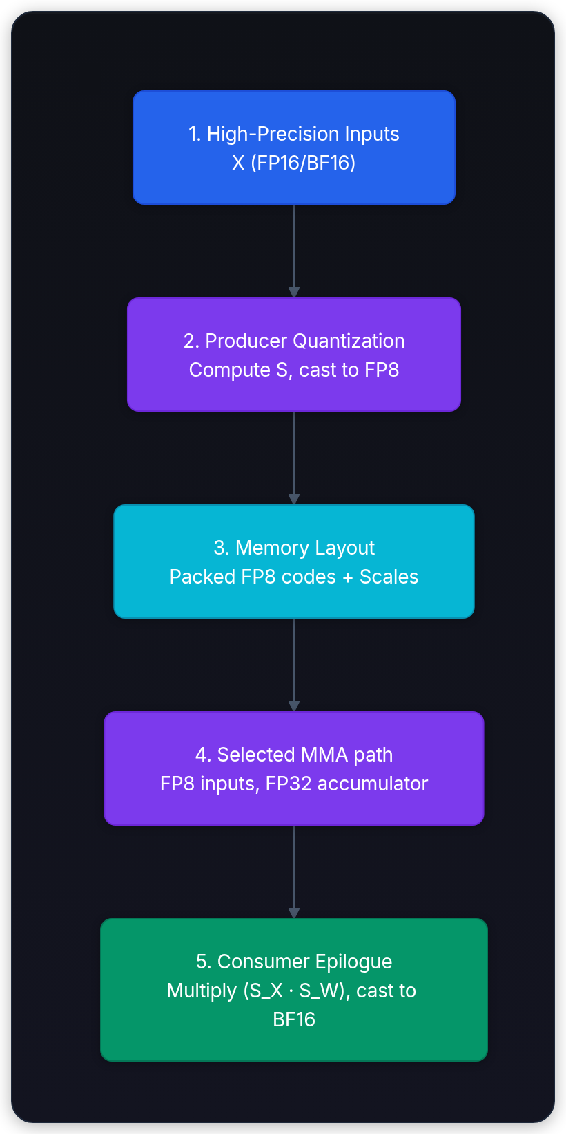
This raises a critical architecture question: who owns quantization and dequantization?

• Quantization is owned by the PRODUCER: The kernel generating the tensor (such as RMSNorm, SiLU, or the prior layer's GEMM epilogue) measures range, computes scale factor $S$, casts values into low-precision codes, and packs both codes and scales into global memory or shared memory (SRAM).
• Dequantization is NEVER a standalone memory-to-memory kernel: Writing an FP32 dequantized tensor back out to DRAM would waste $4\times$ the memory bandwidth and completely erase the speedup of low precision. Dequantization is owned by the CONSUMER GEMM, fused directly into register ALUs during accumulation or epilogue store.

If scaling happens block-wise along the contraction axis $K$ (as in 32-element microscaling with block index $b$):

$$Y_{ij} = \sum_{b=1}^{K/32} \left(S_{X, i, b} \cdot S_{W, j, b}\right) \sum_{k \in \text{block } b} \tilde{X}_{ik} \tilde{W}_{kj}$$

The scale product $(S_{X, i, b} \cdot S_{W, j, b})$ stays inside the outer reduction loop. The Tensor Core accumulates 32-element partial dot products in FP32, multiplies by the block scale product, and sums across blocks.

---

Numerical hazards: subnormals, saturation, and rounding

Running low-precision code exposes three distinct numerical pitfalls. Understanding how they manifest keeps models from silently losing fidelity.

Subnormals and flush-to-zero (FTZ)

Normal floating-point numbers have an implicit leading 1 ($1.f \times 2^{e - \text{bias}}$). Subnormal numbers occur when the exponent bits are all zero; the leading bit drops to 0 ($0.f \times 2^{1 - \text{bias}}$). This allows values to shrink smoothly toward zero, albeit with progressively fewer significant bits.

In OCP E4M3, the smallest positive normal is $2^{-6} = 0.015625$. Subnormals extend down to $2^{-9} \approx 0.001953125$. Under standard round-to-nearest-even (RNE):

• An input of $0.75 \times 2^{-9}$ rounds up to the smallest subnormal $2^{-9}$.
• An input of $0.5 \times 2^{-9}$ lands on an exact tie and rounds down to signed zero (+0.0 or -0.0).

Hardware can introduce another trap: flush-to-zero (FTZ) mode. Some fast matrix instructions or compiler flags flush all subnormals to zero in a single cycle to avoid multi-cycle normalization penalties. If a deep model's residual signals or attention logits drift into the subnormal band, FTZ wipes them out, causing sudden gradient extinction.

Saturation cliffs

What happens when an unscaled or poorly scaled value exceeds the maximum representable magnitude? Under non-saturating conversion, an out-of-range E4M3 value turns into NaN, while an E5M2 value becomes infinity.

Under saturating conversion (the default for production FP8 paths), out-of-range values get clamped to the format limit: $\pm 448$ for E4M3, or $\pm 57,344$ for E5M2.^{[1]Reference 1OCP 8-bit Floating Point Specification (OFP8), Revision 1.0https://www.opencompute.org/documents/ocp-8-bit-floating-point-specification-ofp8-revision-1-0-2023-12-01-pdf-1[5]Reference 5FP8 Conversion and Data Movementhttps://docs.nvidia.com/cuda/cuda-math-api/cuda_math_api/group__CUDA__MATH__FP8__MISC.html}

Saturation creates an artificial flat cliff. A spike of $500$ clamps to $448$; a spike of $50,000$ also clamps to $448$. This destroys relative magnitudes, and in backward passes, the derivative across a clamped plateau is zero, killing parameter updates. Worst of all, saturation produces valid, finite numbers. A production health check that only looks for NaNs and infinities will see clean telemetry while model generations degrade into nonsense.

Rounding: RNE versus stochastic rounding

Standard IEEE and OCP conversion mandates round-to-nearest, ties-to-even (RNE). RNE is deterministic, but it introduces the gradient stagnation trap during low-precision training.

Suppose an optimizer calculates a weight update $\Delta W = -\eta g$. If $|\Delta W|$ is smaller than half of the least significant bit ($\frac{1}{2}\text{LSB}$) of the weight representation, RNE rounds $\Delta W$ down to zero:

$$\operatorname{RNE}(W + \Delta W) = W$$

The weight never updates. Run training for 100,000 steps, and the weight remains frozen in place.

Stochastic rounding breaks this trap by rounding up or down probabilistically based on the distance to the adjacent representable points:

$$\operatorname{SR}(x) = \begin{cases} \lceil x \rceil & \text{with probability } \frac{x - \lfloor x \rfloor}{\lceil x \rceil - \lfloor x \rfloor} \\ \lfloor x \rfloor & \text{with probability } 1 - \frac{x - \lfloor x \rfloor}{\lceil x \rceil - \lfloor x \rfloor} \end{cases}$$

The mathematical expectation of stochastic rounding is strictly unbiased: $\mathbb{E}[\operatorname{SR}(x)] = x$. Even if an update $\Delta W$ equals just $0.01 \times \text{LSB}$, it will round up $1\%$ of the time. Over thousands of iterations, small updates integrate into real weight changes, making training in low precision numerically viable without keeping separate FP32 master copies.

The mandatory FP32 accumulator contract

Never accumulate low-precision products in a narrow format. Consider an inner dimension of $K = 4096$, common in modern LLMs. A single output activation is the sum of 4096 individual products.

If you accumulate in FP16, you hit the swamping boundary quickly. In FP16, once a running partial sum reaches $1024.0$, the gap between adjacent representable numbers is $2^{10-10} = 1.0$. Any individual product smaller than $0.5$ added to that running sum rounds down to zero ($1024.0 + 0.4 = 1024.0$). By the middle of the dot product, the accumulator becomes completely deaf to incoming numbers. Accumulating in FP8 is catastrophic.

Hardware Tensor Cores enforce the Accumulator Contract: inputs are consumed in low precision (FP8, FP16, BF16), multiplication occurs at full or expanded precision, accumulation runs in dedicated 32-bit FP32 registers, and downcasting happens only during the final epilogue store.

---

Hands-on: auditing FP8 conversion boundaries

Let's test subnormal rounding, saturation clamping, and byte-level encoding differences using PyTorch on CPU.

In this script, notice how raw conversion behaves on CPU compared to explicit saturating conversion, and observe how identical raw bytes represent completely different numbers across OCP and FNUZ specifications.

Look at the byte decoding at the end: byte 0x38 decodes to 1.0 in OCP E4M3, but becomes 0.5 in AMD's FNUZ E4M3 because their exponent biases differ (7 versus 8). Byte 0x80 represents negative zero in OCP E4M3, but represents NaN in FNUZ because FNUZ drops signed zeros. Feeding an OCP-encoded buffer into a kernel expecting FNUZ silently alters standard numeric values throughout your model.^{[6]Reference 6Tensor Attributeshttps://docs.pytorch.org/docs/stable/tensor_attributes.html[7]Reference 7Data Types and Precision Supporthttps://rocm.docs.amd.com/en/latest/reference/precision-support.html}

Worked failure: stale delayed scale

Suppose delayed scaling calculates an E4M3 scale factor from a previous iteration's maximum absolute value ($\text{amax} = 10.0$):

$$S_{\text{old}} = \frac{10.0}{448} \approx 0.02232$$

In the current iteration, an activation outlier spikes to $500.0$. The scaled magnitude is:

$$\frac{500.0}{S_{\text{old}}} = \frac{500.0}{10.0 / 448} = 22,400.0$$

Under saturating conversion, $22,400.0$ clamps directly to the format maximum of $448$. During consumer dequantization, reconstruction returns:

$$\hat{x} = 448 \cdot S_{\text{old}} = 448 \cdot \frac{10.0}{448} = 10.0$$

The reconstructed value is finite, positive, and shows no NaN errors, but its relative error is $98\%$. The FP32 accumulator faithfully adds the corrupted product into the running sum, masking the numerical collapse from monitoring systems.

---

Scaling architectures: granularity and delayed scaling

The granularity of your scale factor sets which values compete for the same dynamic range exponent.

The host-device latency dilemma

Calculating an online per-tensor scale requires finding $\text{amax} = \max(|X|)$ across all elements before launching the GEMM:

$$S = \frac{\text{fp8\_max}}{\text{amax}}$$

If a framework calculates this scale on the host CPU, the GPU must write out the maximum, synchronize the CUDA stream, and copy the scalar over PCIe. That introduces a 10 to 50 microsecond pipeline bubble on every single layer.

If the GPU calculates the scale asynchronously using a separate reduction kernel, it avoids CPU synchronization, but it still pays a steep memory bandwidth penalty: the entire tensor $X$ must be read from global memory once to compute amax, and read again by the GEMM kernel.

Delayed scaling in Transformer Engine

NVIDIA Transformer Engine bypasses the reduction pass through delayed scaling.^{[8]Reference 8Using FP8 and FP4 with Transformer Enginehttps://docs.nvidia.com/deeplearning/transformer-engine/user-guide/examples/fp8_primer.html} Instead of measuring the current tensor, it sets the scale factor using an amax history window from prior iterations ($t-1, t-2, \dots$):

$$S_t = \frac{\text{fp8\_max}}{\max_{i \in [1, H]} \text{amax}_{t-i}}$$

While the GEMM executes at step $t$, the kernel computes the actual $\text{amax}_t$ as a side product in register memory and writes it out for future steps. This eliminates both the host synchronization bubble and the extra DRAM read pass.

The risk is scale lag. If an activation spike hits after a distribution shift, the historical scale is too small, causing massive saturation clipping. If the historical maximum was an unusual outlier, the scale remains too large, pushing typical activations down toward the subnormal floor.

Fused online scaling in DeepSeek-V3 and DeepGEMM

Modern open models take a different path. DeepSeek-V3 and its underlying DeepGEMM library reject delayed scaling entirely.^{[9]Reference 9DeepSeek-V3 Technical Report.https://arxiv.org/abs/2412.19437[10]Reference 10DeepGEMM Source Snapshot, July 15 2026https://github.com/deepseek-ai/DeepGEMM/tree/559d79fb6994a58b8a15b4b93bf13ccc16edf247}

Instead of lagging behind history, DeepSeek uses fine-grained block-level scaling ($1 \times 128$ activation tiles and $128 \times 128$ weight tiles). The scale computation is fused directly into the Tensor Memory Accelerator (TMA) load and warp-specialized GEMM pipeline. Scales are evaluated in registers and shared memory as data arrives from global memory, completely avoiding both host synchronization and delayed scale clipping.

Microscaling: the two-row experiment

In OCP Microscaling, every 32-element vector shares an 8-bit scale factor (E8M0). E8M0 stores a pure power-of-two exponent with a bias of 127, encoding scales from $2^{-127}$ up to $2^{127}$. Multiplying by an E8M0 scale in hardware requires zero mantissa multiplication ALUs: it's a simple integer addition to the exponent field!

A 32-value block holds 256 bits of element data plus 8 bits of shared scale, giving an effective payload of:

$$\frac{256 + 8}{32} = 8.25 \text{ bits per element}$$

Let's test our running two-row activation matrix on CPU. Row 0 holds delicate values starting at $0.001$. Row 1 holds an activation spike of $500.0$.

Predict what happens to $0.001$ when it shares one global scale with $500.0$, versus when each row gets its own 32-element block scale:

Follow the numbers closely:

1. Under tensor-wide scaling ($S = 1.116071$): The smallest representable non-zero E4M3 step is $1.116071 \times 2^{-9} \approx 0.00218$. The small activation $0.001$ falls below half of this step and rounds straight to zero. The entire row loses nearly $3\%$ of its dot-product magnitude because an outlier in an unrelated row set the scale.
2. Under block-level scaling ($S_0 = 2^{-8} = 0.00390625$): The first block's scale shifts the dynamic range downward. Its smallest subnormal step becomes $2^{-8} \times 2^{-9} = 2^{-17} \approx 7.63\times10^{-6}$. The small value $0.001$ survives accurately as $0.00097656$ (just $2.3\%$ relative error).
3. Outlier isolation in Row 1 ($S_1 = 2^1 = 2.0$): Row 1 gets its own scale, so its $500.0$ outlier stays confined to its own 32-element chunk without destroying detail in Row 0.

Notice an essential detail in the microscaling specification: a packed row-wise MXFP8 matrix can't simply be transposed in memory to serve as a column-wise operand. In row-wise packing, every 32 elements along the $K$ axis share a scale. In column-wise packing, 32 elements along the $M$ axis share a scale. Transposing the byte buffer groups completely different numbers together under the same scale factor. Both orientations must be quantized independently from higher-precision data.^{[11]Reference 11MXFP8https://docs.nvidia.com/deeplearning/transformer-engine/user-guide/features/low_precision_training/mxfp8/mxfp8.html}

---

Hardware support and kernel ABI contracts

Hardware claims must always be tied to specific GPU microarchitectures, compute capabilities, and driver toolkits.

Before launching a low-precision kernel in production, write out its complete numeric contract:

Treat framework, compiler, and kernel boundaries as strict serialization interfaces. Passing dtype tags, scales, orientation, padding, and accumulator modes together prevents silent numerical drift.

---

Troubleshooting numerical failures

When low-precision outputs diverge from an FP32 reference run, use this diagnostic roadmap:

A reliable incident trace must capture input histograms, amax per scale group, selected scale factors, clip counts, zero counts, accumulator modes, and the profiler-confirmed kernel symbol. Checking only the final output relative error hides where the contract failed.