Personalize this lesson
Adapt explanations and teaching visuals to your background and preferred voice.
The server finishes more requests per second, but users wait longer for the first word. Some streams pause halfway through. A few fast responses contain invalid tool arguments. Has the new build improved?
A single throughput number can't answer that. A useful serving benchmark preserves the incoming workload, measures the client's experience, and counts which responses actually satisfy the task. It must also notice when the load generator, rather than the server, is overloaded.
Continuous Batching and Scheduling explains why prompt processing and generation compete. GPU Profiling, Correctness, and Benchmarking separates kernel timing from broader execution. Here, the boundary moves outward to the client, gateway, and serving system, including failures and waiting time.
The running example is an incident assistant receiving a burst of mixed requests. The downloadable records are explicitly synthetic. They exercise a real local scorer; they aren't observations from a model, a load generator, or a GPU.
Freeze what arrives and when
A workload needs more than an average prompt length. Keep the prompt or token IDs, output policy, request class, and scheduled arrival for each identity. Include the system prompt, retrieved context, and conversation history that the application actually sends.
Consider these six arrivals:
| ID | Scheduled time | Prompt tokens | Output policy | Shared prefix | Class |
|---|---|---|---|---|---|
r01 | 0 ms | 320 | natural stop, cap 96 | runbook A | interactive |
r02 | 120 ms | 336 | natural stop, cap 96 | runbook A | interactive |
r03 | 700 ms | 4,096 | natural stop, cap 256 | none | interactive |
r04 | 760 ms | 280 | natural stop, cap 64 | none | interactive |
r05 | 800 ms | 2,048 | natural stop, cap 512 | policy B | background |
r06 | 1,900 ms | 480 | natural stop, cap 128 | runbook A | interactive |
The long prompt at r03 can interfere with the short request arriving 60 ms later. r05 may occupy a decode slot for longer. Prefix reuse can reduce work, but only if the runtime supports it and the cache state permits a hit. Repeating one prompt isn't inherently wrong; it's wrong to represent a cache-friendly test as an unrelated production mix.
Count tokens with the pinned tokenizer and chat template. An output cap isn't an observed output length. Keep both. Forcing exact output lengths, for example by ignoring end-of-sequence (EOS) tokens, can isolate scheduler behavior, but that is a shape-controlled stress test rather than a natural-response quality evaluation.
Generate the realized trace once, save it, and hash the exact bytes. A seed alone doesn't guarantee identical rows across library or tokenizer versions. The six-row download later contains only scheduling metadata, not these prompts; it's a scorer fixture, not a complete workload for replay against an endpoint.
Public traces can help challenge assumptions. BurstGPT reports real arrival and token-length patterns; ServeGen models production workload characteristics with per-client arrival and request-data models.[1][2] Neither makes its traffic representative of your users. Preserve length tails, prompt/output correlation, tenant mix, prefix reuse, and conversation dependencies that matter to your application.
Don't let a slow server turn down its own test
An open-loop generator schedules requests independently of completions. If r04 is due at 760 ms, r03 still running doesn't cancel that arrival.
A closed-loop generator starts another request when a virtual user becomes free. When responses slow down, its offered rate falls. That is appropriate for studying a fixed user population, but it answers a different question from capacity under an external arrival rate.
| Mode | What controls arrivals | Suitable question |
|---|---|---|
| Open-loop | Stored timestamps or an independent clock | Can the system sustain this offered workload? |
| Closed-loop | Completions and user think time | What do this many active users experience? |
| All-at-once | Every request released at the start | How does the system handle a batch or admission burst? |
MLPerf Inference formalizes different scenarios: Single Stream waits for each completion, while Server/Interactive uses Poisson arrivals. Its quality and latency rules are part of a defined benchmark, not labels a custom load test can borrow.[3]
Rate, concurrency, and burstiness aren't interchangeable
In a stable system, Little's Law relates average outstanding requests , admitted arrival rate , and mean time in the same system :[4]
At 3 requests/s and 0.9 seconds average latency, the average outstanding count is 2.7. A client capped at two outstanding requests can't sustain that combination. Even a cap of three may throttle bursts: an average isn't a maximum. Check whether the cap actually binds.
A Poisson process has exponential inter-arrival gaps with coefficient of variation . Regular spacing has . Real traffic can have correlated bursts that neither description captures. Save realized timestamps when replay identity matters.
As checked on October 10, 2026, vllm bench serve exposes --request-rate, --burstiness, and --max-concurrency. Its burstiness is a Gamma shape parameter , with : values below one make gaps more variable. Infinite request rate is an all-at-once or concurrency-limited stress mode, not a finite-rate open-loop test. For production server benchmarking, the current vLLM guide recommends GuideLLM; the built-in benchmarks focus primarily on feature evaluation and regressions.[5]
Inspect the realized schedule too: the current implementation's constant-rate path rescales sampled gaps so the final scheduled arrival is at request count divided by rate. That finite trace isn't an unconditioned Poisson realization. Self-timed replay instead uses stored timestamps and bypasses rate, burstiness, and ramp-up controls.[6]
Time-scaling a stored trace is one way to sweep offered rate while preserving order and relative gaps. It also compresses the duration of a fixed-size cohort. Either extend the trace to keep measurement duration comparable or report that changed duration; you can't claim both fixed request count and fixed duration while changing the rate.
Measure the generator's lateness
Keep scheduled_ms and sent_ms in a common client monotonic-clock domain. If a request is scheduled at 760 ms but sent at 1,100 ms, the generator is 340 ms late. Measuring only from send time hides that discrepancy.
Report send-relative latency and scheduled-relative delay separately. Declare a schedule-lag tolerance and invalidate capacity evidence when the generator can't reproduce the offered load. Delayed or unsent requests must not disappear from the workload denominator. This is one form of coordinated omission: the test stops observing the work that should have arrived during a slowdown.
Current vLLM supports client_queue_time in --percentile-metrics when a client concurrency cap creates a wait. With a finite request rate and a client cap, e2el_including_client_queue adds that wait to the adapter's reported latency. It doesn't independently measure scheduler lateness or extend the adapter's end boundary to terminal completion. That metric is omitted for infinite request rate. These summaries cover successful requests; they don't replace offered-request failure accounting. A client queue measures its own backpressure; use server spans to attribute a separate server queue.[6]
Client and server clocks aren't automatically comparable. Use client timestamps for client latency. Use server-local spans for queueing and compute attribution, or a measured clock-synchronization scheme when joining absolute times across machines.
A client cap of two binds while testing a target of 3 requests/s. The server's measured latency remains low. What does that establish?
Answer
It establishes behavior under the throttled workload, not capacity at 3 requests/s. Keep the delayed arrivals, report schedule lag, and rerun with a generator that can sustain the intended schedule.
Give the run an arrival window and a drain policy
Separate readiness, warmup, measurement, and drain. Warmup may include loading, kernel compilation, CUDA Graph capture, connections, and scheduler initialization. Don't populate prefix caches unless the measured scenario is supposed to begin with those entries warm.
During the measurement arrival window, send the declared workload. When arrivals stop, retain every request until terminal success, rejection, cancellation, error, or timeout. Choose timeouts before the run. A late response doesn't retroactively undo an earlier timeout experienced by the client.
There are two useful but different accounting views:
- An arrival cohort includes requests scheduled in a half-open window such as
[0, 2000)ms. Judge all of their outcomes, including those observed during drain. - A wall-clock interval counts completions occurring inside that interval, regardless of when those requests arrived. Track starting and ending outstanding work to interpret it.
Don't divide one population by the other population's elapsed time. For the local exercise, cohort rates use elapsed time from arrival-window start through the later of window end and last terminal outcome. Those finite-run rates include drain and aren't sustainable-capacity estimates.
For sustained load, inspect outstanding work over time and compare admitted, completed, rejected, and timed-out rates. A flat server queue alone isn't enough: aggressive rejection can keep it flat while users fail. Repeat sufficiently long runs to observe relevant warmup, cache, thermal, and traffic cycles.
Time what the protocol actually reveals
Let be client send time, first output-token time, final output-token time, and terminal completion time. Assume these token events genuinely have token granularity and use the same clock.
Time to first token (TTFT) measures the initial wait. Inter-token latency (ITL) measures each subsequent gap:
For , request-mean time per output token (TPOT) is:
End-to-end completion latency is:
The final token can precede the terminal event, usage metadata, or connection completion. Replacing with silently changes the metric to last-token latency.
For a request sent at zero, token times [240, 280, 320, 440, 480] ms and terminal time 500 ms produce TTFT 240 ms, TPOT 60 ms, and E2E 500 ms. The four gaps are [40, 40, 120, 40] ms. One 120 ms pause is hidden inside the 60 ms mean.
The following calculation checks those definitions. It doesn't run inference.
from math import ceil

tokens = [240, 280, 320, 440, 480]
sent, terminal = 0, 500
assert sent <= tokens[0] <= tokens[-1] <= terminal
gaps = [b - a for a, b in zip(tokens, tokens[1:])]
assert all(gap >= 0 for gap in gaps)
print(f"TTFT: {tokens[0] - sent} ms")
print(f"ITL: {gaps} ms")
print(f"TPOT: {sum(gaps) / len(gaps):.0f} ms")
print(f"last-token latency: {tokens[-1] - sent} ms")
print(f"terminal E2E: {terminal - sent} ms")
print(f"nearest-rank p99 of four gaps: {sorted(gaps)[ceil(.99 * len(gaps)) - 1]} ms")TTFT: 240 ms
ITL: [40, 40, 120, 40] ms
TPOT: 60 ms
last-token latency: 480 ms
terminal E2E: 500 ms
nearest-rank p99 of four gaps: 120 msFor one-token output, there are no inter-token intervals. TPOT is undefined, not zero. Define the eligibility rule before scoring. The supplied scorer treats the TPOT criterion as not applicable for a successful single-token response, while still checking TTFT and quality. An empty successful output is invalid under this lesson's text-response contract; another endpoint might legitimately define empty output differently.
A streaming chunk isn't necessarily a token
A server-sent event (SSE) may contain several tokens, metadata without text, or a fragment whose tokenization depends on later text. TCP reads aren't SSE event boundaries either. An adapter must reconstruct the protocol, recognize its terminal/error events, and preserve timestamps before producing normalized records.
| Observation | Honest metric | What it doesn't prove |
|---|---|---|
| First response byte | Time to first byte | That output text has started |
| First content-bearing chunk | Time to first content chunk | Exact first-token emission time |
| Client text chunks | Inter-chunk latency | Individual token ITL |
| Server token events | Server token cadence | Client-visible network cadence |
| Client token-granular events | Client-observed ITL | GPU kernel duration |
Dividing a multi-token chunk's delay by its token count invents arrival times. Keep chunk metrics when those are the available observations. The downloadable scorer accepts normalized token events; it isn't an SSE parser and can't manufacture missing granularity.
For example, vLLM calls gaps between accepted stream events ITL, even when speculation puts several tokens in one event. Its request TPOT amortizes the adapter's reported latency minus TTFT over output tokens minus one. As checked on October 10, 2026, the pinned Completions and Chat Completions adapters end that latency at the last event with nonempty choices, which can carry empty content. Later usage-only events and [DONE] don't extend it. The Responses adapter instead timestamps text and reasoning deltas. These boundaries don't necessarily measure terminal completion or first visible text.[7][6]
This lesson's token-granular worksheet uses the first-to-last token interval and records terminal completion separately. Match the endpoint, observed events, token-count source, and installed adapter version before comparing those numbers.
Smoothness needs the order of events
A long gap isn't always a playback stall. Earlier tokens can arrive ahead of a reading cadence and provide slack. Etalon's fluidity metric uses token deadlines to capture this distinction.[8]
For a simple illustration, set a first-token deadline of 300 ms and a cadence of 80 ms. Deadlines for five tokens are [300, 380, 460, 540, 620]. The earlier example meets all five even though one raw ITL is 120 ms. In [300, 380, 460, 580, 620], the fourth token misses its deadline despite mean TPOT being 80 ms.
This illustrates why deadline and gap metrics answer different questions. Etalon also counts how many playback deadlines a stall crosses, then resets future deadlines after the late token. A long stall can contribute several missed deadlines, so its fluidity index isn't simply the fraction of late observed tokens. Don't substitute this five-token comparison for its algorithm or for a measured reading-speed requirement.[8]
Keep the denominator visible
Define a request as qualified only when it has terminal success, acceptable output, and the declared latency properties. HTTP 200 or valid JSON alone doesn't establish task correctness. Errors, timeouts, rejected requests, unsent requests, and wrong answers stay in the offered-request denominator.
Two quantities are often both called goodput:
This is a rate of useful completed work for a specified population and interval. A capacity boundary asks which offered rate still meets the declared service-level objective (SLO):
Here is qualified requests divided by all offered requests, and is the required attainment. DistServe uses a goodput definition tied to the maximum rate satisfying TTFT/TPOT attainment requirements per GPU.[9] Name your definition instead of assuming every tool's “goodput” means that capacity boundary.
A system may finish more qualifying requests per second while also failing a larger fraction of incoming requests. Useful-work rate alone then improves, but a 95% attainment promise fails. Divide a fleet rate by GPU count only when comparing a fixed, stated resource allocation.
Run a strict local scorer
Download the scorer, the synthetic scheduling manifest, and the synthetic outcomes into one directory. Python 3.12 or newer and uv are sufficient. There are no model downloads, endpoint calls, or third-party Python dependencies.
uv run score_requests.py example-trace.json example-events.jsonl > scored.jsonSave the accounting tests beside those files and run uv run test_score_requests.py. They exercise timing, missing and duplicate outcomes, failure denominators, single-token output, malformed records, and CLI exit codes. Passing them checks the scorer, not a serving system.
The manifest fixes six IDs and scheduled times in [0, 2000) ms. Each JSONL outcome has this shape:
{
  "id": "r01",
  "sent_ms": 0,
  "terminal_ms": 500,
  "token_ms": [240, 280, 320, 440, 480],
  "status": "success",
  "quality_pass": true
}
quality_pass is a supplied task judgment. The scorer doesn't judge semantics. Its input validation checks exact fields, finite nonnegative timestamps, temporal ordering, unique IDs, and a terminal outcome for every expected request. Unknown IDs, missing outcomes, duplicate JSON keys, nonfinite values, and empty successful outputs are errors. Equal token timestamps are allowed because the measuring clock can have finite resolution.
The supplied outcomes exercise different branches:
| Request | Outcome | Qualified? |
|---|---|---|
r01 | TTFT 240 ms, TPOT 60 ms, terminal E2E 500 ms | Yes |
r02 | Single token, TTFT 170 ms; TPOT not applicable | Yes |
r03 | TTFT 340 ms exceeds the 300 ms limit | No |
r04 | TTFT 285 ms and TPOT 61 ms | Yes |
r05 | Fast successful response, but supplied quality judgment fails | No |
r06 | Partial output followed by timeout at 2,500 ms | No |
All six count toward attainment, giving 3 / 6 = 50%. There are five protocol successes, not six. The cohort horizon is 2.5 seconds, giving 2.0 successful requests/s and 1.2 qualified requests/s. The arrival window is two seconds, giving a realized offered rate of 3.0 requests/s. These denominators are printed separately.
The report includes exact input hashes, per-request metrics, and successful-request-only percentile populations. Failed requests remain in attainment even though their partial streams don't enter successful-latency percentiles. capacity_estimate_rps is deliberately null: these records contain neither a sustained run nor a capacity sweep.
Exit code zero means the input and schedule checks passed, not that a deployment is approved. Code 2 means the accounting is available but a request was unsent or schedule lag exceeded 20 ms. Code 1 means malformed or incomplete inputs. Preserve nonzero exits in automation; don't let a successful tee hide them.
Try three changes in a copy of the JSONL file:
- Delete
r06. The scorer must reject the incomplete cohort instead of improving attainment by dropping a timeout. - Mark
r05as quality-passing. Attainment becomes four of six; the parser is trusting a changed judgment, not discovering better model quality. - Change
r04.sent_msfrom 765 to 800. Its measured TTFT falls to 250 ms, but schedule lag rises to 40 ms and the run becomes invalid for its declared load.
For an unsent request, retain its ID with status not_sent, null sent_ms, no tokens, a terminal accounting time, and quality_pass: false. If the client retries requests, keep attempt-level records and a separate logical-request result; this small schema deliberately rejects duplicate IDs rather than silently merging retries.
Find a boundary without overstating the evidence
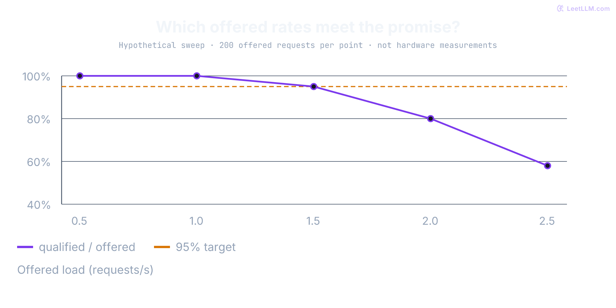
The hypothetical sweep below illustrates selection logic. The inputs are supplied observations, not results from the six-request parser fixture or any hardware run. Require 95% attainment, at most 20 ms schedule lag, and no sustained backlog growth.
| Offered RPS | Qualified / offered | Attainment | Max schedule lag | Backlog trend | Point estimate passes? |
|---|---|---|---|---|---|
| 0.5 | 200 / 200 | 100% | 8 ms | flat | Yes |
| 1.0 | 200 / 200 | 100% | 9 ms | flat | Yes |
| 1.5 | 190 / 200 | 95% | 11 ms | flat | Yes |
| 2.0 | 160 / 200 | 80% | 12 ms | growing | No |
| 2.5 | 116 / 200 | 58% | 16 ms | growing | No |
Under these arithmetic rules, 1.5 RPS is the highest passing tested point. It isn't a proven maximum between points, a statistically certified 95% service level, or a safe production target. Repeat and refine the boundary, test the failing neighbor, and select operating margin for failures and traffic drift.
A percentile needs a population and enough observations
Nearest-rank p95 of 20 values selects the 19th ordered value. Nearest-rank p99 of 80 gaps selects the maximum. Those are reproducible calculations, not precise estimates of a production tail.
Pooled ITL percentiles give longer responses more weight because they contribute more gaps. A percentile across per-request worst gaps answers a different question. Neither can be recovered by averaging percentile summaries from separate runs. Keep raw samples, state the convention, and stratify meaningful prompt-length, output-length, and priority classes.
The same caution applies to attainment: observing 190 successes in 200 trials doesn't establish that the underlying pass probability is at least 95%. Predeclare an uncertainty rule and minimum evidence. For correlated traffic, resample whole runs or suitable time blocks rather than pretending each token gap is an independent sample. Repeating an unrepresentative trace can't repair its missing workload classes.
What does 190 of 200 actually support?
Suppose, for this calculation, that request outcomes are independent Bernoulli trials with a constant pass probability at one preselected load. A one-sided 95% Wilson lower confidence bound is below the observed proportion. NIST documents this method and distinguishes it from a simple symmetric normal interval.[10]
from math import sqrt
from statistics import NormalDist

z = NormalDist().inv_cdf(.95)
for good, n in [(190, 200), (200, 200), (20, 20)]:
    observed = good / n
    lower = (
        observed + z*z/(2*n)
        - z*sqrt(observed*(1-observed)/n + z*z/(4*n*n))
    ) / (1 + z*z/n)
print(f"{good}/{n}: observed {observed:.1%}; one-sided 95% Wilson lower {lower:.1%}")190/200: observed 95.0%; one-sided 95% Wilson lower 91.8%
200/200: observed 100.0%; one-sided 95% Wilson lower 98.7%
20/20: observed 100.0%; one-sided 95% Wilson lower 88.1%The first row passes the 95% point-estimate rule but fails a rule requiring that lower bound to reach 95%. Even twenty perfect outcomes don't pass that stronger rule. Confidence describes the interval procedure's coverage under its assumptions; it isn't the fraction of requests meeting the SLO or a 95% posterior probability about this particular interval. Choosing the best point after many noisy sweeps needs a selection-aware procedure or fresh confirmation runs. Shared bursts can invalidate the independent-trial calculation.
Alternate baseline and candidate run order. Keep cold-start and warm-capacity results separate, and consider a downward sweep when cache or thermal history creates hysteresis. Don't select the best of many noisy runs and omit the others.
Join performance and quality before release
Performance and quality need linked but distinct evidence. Check every performance response for protocol completion, finish reason, actual output length, and required schema. Use a stable task suite for factual support, correct tool arguments, abstention, and other semantic requirements.
A short answer produced by accidental truncation can look faster. A valid speculative decoder should preserve its target sampling distribution under its stated assumptions; “uses speculation” isn't itself evidence of degraded quality. Still verify the implemented combination, including stop handling and output parsing, rather than assuming that a faster engine preserved the task.
If semantic quality is evaluated only on a separate sampled suite, don't label every unscored performance request semantically qualified. Report performance attainment and the separate quality acceptance result. A per-request quality_pass field needs actual per-request evidence for that stronger claim.
Keep a compact record of:
- Model, tokenizer, template, quantization, engine, client, and image identities.
- Hardware count, placement, drivers, gateway/network scope, and relevant limits.
- Exact workload bytes, realized timestamps, warmup/cache policy, timeouts, and run duration.
- All terminal outcomes, raw timing events, quality judgments, and system telemetry.
- Metric populations, denominators, thresholds, uncertainty rules, repetitions, and rejected runs.
- Selected operating margin, recovery plan, and conditions that weren't tested.
A hash binds bytes, not truth. A successful parser proves that records satisfy its schema and arithmetic rules, not that they were collected faithfully. Preserve original logs and measurement provenance so another engineer can inspect that boundary.
The report shows good attainment, flat queue depth, and exit code zero. Can you approve the serving configuration from that alone?
Answer
No. Check whether the load was reproduced, failures and rejections were retained, the workload and quality evidence are representative, and the run is long and repeatable enough to support the claim. The local scorer intentionally doesn't infer capacity or approve a deployment.