Personalize this lesson
Adapt explanations and teaching visuals to your background and preferred voice.
A latency model predicts that the next request will finish in 40 milliseconds. Should a caller rely on a 50-millisecond deadline? A prediction interval such as [32, 48] adds information the point prediction lacks, but even that range isn't a promise about this particular request.
Statistical Learning and Generalization established why untouched evidence matters. Here the target changes: a confidence interval estimates a population quantity, such as mean latency; a prediction interval covers a new outcome. Split conformal prediction uses a held-out calibration split to turn a frozen predictor's errors into prediction sets without assuming Gaussian noise. Heavy tails alone do not prevent the guarantee. Bursty dependence and changing traffic can, because conformal prediction still needs a sampling assumption.[1]
Under an exchangeability condition on the data, split conformal prediction guarantees that future outcomes fall inside the prediction set with at least a chosen probability:
Here is the allowed miscoverage rate, such as for an 80% target. The probability averages over both calibration data and the new outcome, conditional on an independently fitted procedure. The rule is valid for any positive calibration size , but a small sample can force an uninformative set such as the entire outcome space.
All latency values below are synthetic teaching data. We start with predictions already made by a frozen model; this lesson calibrates their uncertainty rather than fitting another predictor.
Freeze the model before measuring its errors
Before calculating a radius, decide which rows are allowed to influence it. Three slices play different roles:
| Split | Role | Prohibited shortcut |
|---|---|---|
| Training | Fit the latency model | Report training residuals as independent calibration |
| Calibration | Measure errors from the already-frozen model | Tune the model repeatedly against calibration outcomes |
| Test or deployment | Check interval coverage on new requests | Include those outcomes in the original coverage claim |
Keep calibration examples out of fitting and model selection, including preprocessing and scale estimation. Choose the prediction procedure and score rule independently of that split. Model selection can use separate validation data within the training workflow. Calibration then selects the score threshold; it does not retune the predictor.
For a 40-millisecond prediction, an observed 44 milliseconds gives an error of 4; an observed 53 gives an error of 13. A simple regression nonconformity score records that miss as the absolute residual . Larger scores mean the point prediction missed by more.
The finite-sample guarantee relies on exchangeable calibration and future examples, conditional on the fitted procedure: their joint distribution is unchanged by permuting their positions. Formally, for calibration points and one future test point:
for every permutation , where and equality in distribution is denoted by . Independent draws from the same distribution satisfy this condition; exchangeability is more general than independence. A queueing time series, diurnal traffic swings, or altered prompt distribution may not satisfy it. Shuffling an already shifted log does not restore the required joint law.[2]
A model was repeatedly tuned using the same nine examples later labeled as its calibration split. Why can't their residuals support the ordinary split-conformal guarantee?
Answer
Those outcomes influenced the model before calibration, so their residuals are no longer held-out measurements of a frozen predictor. Their apparent errors can be optimistically small, and the ordinary exchangeability argument for fresh request outcomes no longer follows.
Let nine errors choose the radius
Our nine held-out requests produce these sorted absolute errors, measured in milliseconds. Which position should set the radius for the next request?
For 80% target coverage, allow a miscoverage rate of . With nine calibration errors plus one future error, there are ten possible rank positions. Covering the first eight positions gives 8/10 = 80%. The correction counts the future request as well as the calibration requests.
In general, with calibration size , select the following residual quantile. Its order statistic, the value at a numbered position in the sorted sample, has rank:[1]
The ceiling brackets mean round upward. For example, an 85% target would require , not eight. At our 80% target, rank eight selects an 8 ms error. Call this selected radius . A new prediction of 40 milliseconds therefore gets:
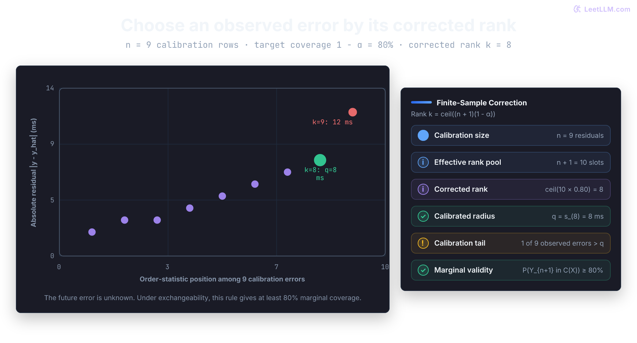
The next cell constructs the absolute errors from frozen predictions and outcomes. Its helper selects an observed order statistic directly, avoiding interpolation between two residuals. Python index rank - 1 converts the one-based rank to a zero-based list position.
from math import ceil, inf, isfinite

def conformal_radius(scores, coverage):
    if not 0 < coverage < 1:
        raise ValueError("coverage must be strictly between 0 and 1")
    ordered = sorted(scores)
    if not ordered or any(not isfinite(s) or s < 0 for s in ordered):
        raise ValueError("provide nonempty, finite, nonnegative scores")
    rank = ceil((len(ordered) + 1) * coverage)
    radius = ordered[rank - 1] if rank <= len(ordered) else inf
    return rank, radius

cal_predictions = [30, 35, 40, 45, 50, 55, 60, 65, 70]
cal_observed = [32, 32, 43, 41, 55, 49, 67, 57, 82]
residuals = sorted(abs(actual - guess)
                   for guess, actual in zip(cal_predictions, cal_observed, strict=True))
rank, radius = conformal_radius(residuals, coverage=0.80)
prediction = 40

print("sorted absolute errors:", residuals)
print(f"corrected rank: {rank} of {len(residuals)}")
print(f"calibration radius: {radius} ms")
print(f"prediction interval: [{prediction - radius}, {prediction + radius}] ms")sorted absolute errors: [2, 3, 3, 4, 5, 6, 7, 8, 12]
corrected rank: 8 of 9
calibration radius: 8 ms
prediction interval: [32, 48] msAn implementation trap: a library quantile convention is not necessarily an order-statistic index. NumPy's method="higher" uses its own position formula. Feeding it level returns the ninth residual here, not the eighth. That radius is conservative in this example, but differs from the intended rule. Direct selection makes the rank explicit:[3]
import numpy as np

scores_array = np.array(residuals)
desired_rank = 8
direct = np.partition(scores_array, desired_rank - 1)[desired_rank - 1]
higher = np.quantile(scores_array, desired_rank / len(scores_array), method="higher")
print(f"direct eighth order statistic: {direct}")
print(f"NumPy higher quantile at 8/9: {higher:g}")direct eighth order statistic: 8
NumPy higher quantile at 8/9: 12The helper returns inf when the requested rank exceeds the available scores. That's deliberate, not a numerical failure. At 90% coverage the ninth error gives radius 12; at 95% the required rank is ten. The standard rule then uses , giving the entire real line rather than inventing a tenth error.[1]
Check the boundary in code. Raising the target can only preserve or widen the interval:
for coverage in (0.80, 0.90, 0.95):
    rank, q = conformal_radius(residuals, coverage)
print(f"target={coverage:.0%} rank={rank} radius={q} width={2*q}")target=80% rank=8 radius=8 width=16
target=90% rank=9 radius=12 width=24
target=95% rank=10 radius=inf width=infDon't clip rank ten to nine: a largest-of-nine threshold supports a 90% lower bound in the no-ties case, not 95%. With 19 calibration errors, 95% first becomes possible with a finite observed threshold: . That's a mathematical minimum, not a recommendation for a stable calibration sample. Known bounds on the outcome could support other finite sets; the unavailable threshold here is specific to this residual-quantile construction.
Why does the example choose the eighth residual instead of simply multiplying nine by 0.8 and rounding down?
Answer
The finite-sample conformal rank is ceil((n+1)(1-alpha)). For nine calibration rows and 80% coverage, that is ceil(10 times 0.8), which selects the eighth order statistic.
Why the extra rank gives coverage
Temporarily imagine ten distinct scores, one from the future request and nine from calibration. Exchangeability makes the future request equally likely to occupy any of the ten sorted positions. Its score is no larger than the eighth calibration score exactly when it lands in positions one through eight.
You can inspect every possible test position without a random simulation. The following scores are a separate rank-only example, not additional latency measurements. Each pass holds out one score and calibrates on the remaining nine:
scores = list(range(1, 11))
covered_positions = []

for index, test_score in enumerate(scores):
    calibration = scores[:index] + scores[index + 1:]
    _, q = conformal_radius(calibration, coverage=0.80)
    if test_score <= q:
        covered_positions.append(index + 1)

print("covered test ranks:", covered_positions)
print(f"covered positions: {len(covered_positions)}/{len(scores)}")covered test ranks: [1, 2, 3, 4, 5, 6, 7, 8]
covered positions: 8/10Our latency fixture has tied errors at 3 ms. Ties don't invalidate the lower coverage bound when the set includes the boundary (score <= q); they can make coverage conservative. Don't discard tied rows or promise exact 80% coverage. When scores are almost surely distinct (continuous nonconformity scores), conformal prediction also provides a tight upper bound on coverage:
For the unmodified rank rule with almost surely distinct scores, coverage is exactly : here . The displayed 80–90% bound is a looser general expression. With ties, only the lower bound is assured; for example, all scores equal to zero can give 100% coverage. Neither statement conditions on the particular realized calibration sample. Predictor quality affects interval usefulness, even when the rank guarantee remains valid.[4]
Watch coverage appear in new requests
The interval [32, 48] covers an actual 44-millisecond outcome and misses 53 milliseconds. That single request tells us what the rule does, not whether the rule is reliable. Coverage is measured across a stream of new comparable examples.
Keep the 80% radius 8 fixed and inspect four new synthetic request outcomes. Each request has its own interval centered at its prediction. Before running the cell, predict which outcome falls outside.
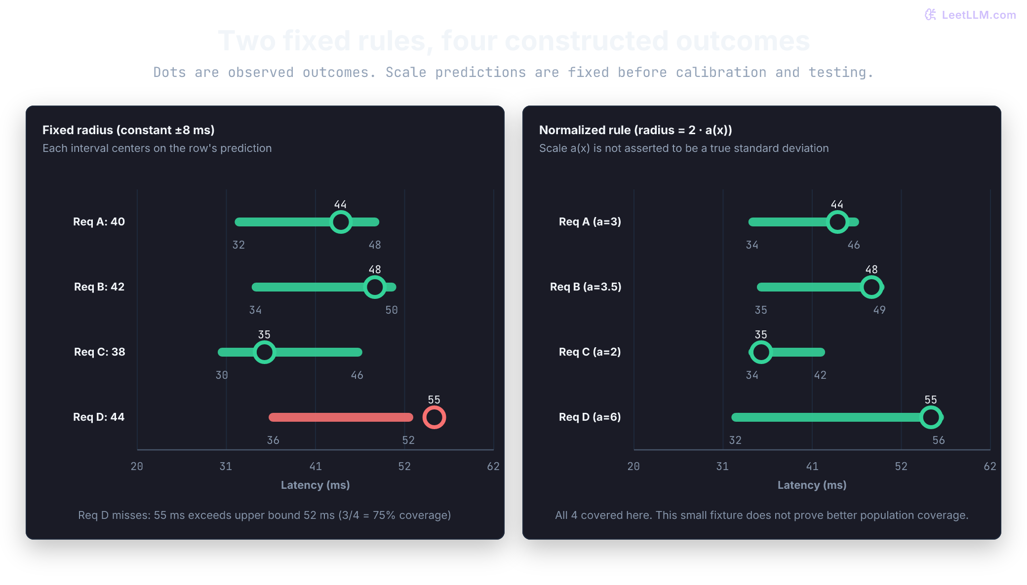
predictions = [40, 42, 38, 44]
observed = [44, 48, 35, 55]

covered = [abs(actual - guess) <= radius
           for guess, actual in zip(predictions, observed, strict=True)]
for guess, actual, is_covered in zip(predictions, observed, covered):
    print(f"predicted={guess} actual={actual} covered={is_covered}")

print(f"observed coverage: {sum(covered)}/{len(covered)}")
print(f"interval width: {2 * radius} ms")predicted=40 actual=44 covered=True
predicted=42 actual=48 covered=True
predicted=38 actual=35 covered=True
predicted=44 actual=55 covered=False
observed coverage: 3/4
interval width: 16 msA four-row observed coverage of 75% doesn't contradict an 80% marginal coverage guarantee. Four requests are a noisy sample, so the observed fraction can move around the target.
Two sources of variation exist: this calibration sample selected one particular radius, and the four test outcomes are another small sample. Even a very long test run with that fixed radius needn't achieve the nominal coverage. Standard split conformal isn't a guarantee conditional on one realized calibration set.[1]
Classification nonconformity scores and adaptive prediction sets
Conformal prediction isn't limited to regression intervals. In multiclass classification, the output is a set of candidate classes guaranteed to contain the true label with probability at least .
Different nonconformity scores produce different set behaviors:
- Naive softmax score: Let denote the model's estimated probability for class . The score is . After computing threshold on calibration data, the prediction set includes all classes whose predicted probability is at least :
When a query is ambiguous and the model distributes probability thinly across many classes (for example, four classes near 0.25), no single class may exceed . That produces an empty prediction set .
- Cumulative scores used in Adaptive Prediction Sets (APS): Let be class labels sorted by descending model output, with a fixed tie rule, and let be their probabilities. If , the deterministic cumulative score is:[5]
Calibrate this score using its own held-out true labels. Direct inversion gives . This can be empty when even the top class probability exceeds .
A simple conservative variant includes labels through the first cumulative sum strictly greater than , or all labels if no crossing exists:
This is a nonempty superset of the directly inverted set, so it preserves the lower coverage guarantee while potentially increasing size. A randomized APS construction can remove the crossing class, sometimes producing an empty set; its calibration must match that randomized score.[5] Model outputs need not be calibrated probabilities for conformal validity, and set size alone does not establish correctness.
Try two new inputs after calibrating on nine constructed rows whose true class is class 0. All outputs are fixed teaching fixtures, not fitted or audited classifiers:
def cumulative_scores(probabilities):
    order = sorted(range(len(probabilities)), key=lambda c: (-probabilities[c], c))
    mass = 0.
    scores = {}
    for label in order:
        mass += probabilities[label]
        scores[label] = mass
    return order, scores

cal_top = [.55, .60, .65, .70, .75, .80, .85, .90, .95]
cal_probabilities = [[p, (1-p)/3, (1-p)/3, (1-p)/3] for p in cal_top]
_, q_soft = conformal_radius([1-row[0] for row in cal_probabilities], .80)
_, q_aps = conformal_radius([cumulative_scores(row)[1][0]
                            for row in cal_probabilities], .80)
print(f"softmax threshold score: {q_soft:.2f}")
print(f"cumulative threshold score: {q_aps:.2f}")

for name, probabilities in [("confident", [.98, .01, .005, .005]),
                            ("ambiguous", [.25, .25, .25, .25])]:
    order, scores = cumulative_scores(probabilities)
    naive = [c for c in order if 1-probabilities[c] <= q_soft]
    base = [c for c in order if scores[c] <= q_aps]
    conservative = []
    for label in order:
        conservative.append(label)
        if scores[label] > q_aps:
            break
    assert set(base) <= set(conservative)
print(f"{name}: naive={naive} cumulative={base} conservative={conservative}")softmax threshold score: 0.40
cumulative threshold score: 0.90
confident: naive=[0] cumulative=[] conservative=[0]
ambiguous: naive=[] cumulative=[0, 1, 2] conservative=[0, 1, 2, 3]Does every APS implementation guarantee nonempty prediction sets?
Answer
No. Direct inversion of cumulative-through-label scores can be empty, and randomized APS can remove the crossing label. The conservative superset shown here is nonempty by construction. Its larger sets retain the lower marginal coverage guarantee, not exact coverage or certainty about their labels.
Find the traffic the average hides
The four-row result measures overall empirical coverage. Breaking that count down by request type asks a different question: who receives the misses?
That guarantee isn't conditional coverage for every subgroup or individual feature value. Consider a constructed evaluation report with 750 short and 250 long requests. Short requests have 96% coverage; long requests have only 54%. The weighted average still exceeds 80%:
These are hypothetical counts, not results from the four-request test above. They expose what an aggregate metric can hide. If the mix shifted to half short and half long while those subgroup rates stayed the same, overall coverage would fall to 0.5 * 0.96 + 0.5 * 0.54 = 75%. The old population guarantee wouldn't transfer automatically to that new mix.[2]
An 80% conformal target passes across all traffic, but long requests are covered only 54% of the time. Does the population-wide guarantee refute the long-request measurement?
Answer
No. Standard split conformal guarantees marginal coverage across the exchangeable population, not equal conditional coverage for every prompt-length subgroup. A common well-covered group can keep the aggregate above target while a smaller long-request group remains unsafe.
Different failures call for different repairs:
| Failure | Symptom | Appropriate response |
|---|---|---|
| Model trained on calibration rows | Residuals look too small | Refit with a genuinely separate calibration split |
| Prompt lengths shift after launch | Recent interval misses cluster on long prompts | Investigate the shift; fresh calibration helps only if its assumptions fit subsequent traffic |
| Tenant-specific error differs | Overall coverage passes while one tenant fails | Measure subgroup coverage; consider separately calibrated, predefined groups |
| Noise grows with request size | Constant intervals are too narrow for large requests | Use normalized nonconformity scores or group-aware methods |
| Calibration sample is tiny | Desired rank exceeds available observations | Gather more data or acknowledge an unbounded set |
Constant width is not the only option. A second frozen model can predict a positive scale in milliseconds. This need not equal the true conditional standard deviation. Calibrate the dimensionless scores , then use . Both models and the score rule must be fixed independently of calibration. The method changes width adaptation; it does not produce exact conditional coverage.[4]
For the right side of the figure, use the following prespecified synthetic scale outputs. They are not inferred from calibration labels or chosen to repair the four test misses. The same held-out rows can calibrate different fixed score rules, but selecting a favorite afterward would need its own selection analysis or fresh calibration:
cal_scales = [2, 2, 2, 2, 3, 3, 4, 4, 4]
normalized = [abs(actual - guess) / scale
              for guess, actual, scale in
              zip(cal_predictions, cal_observed, cal_scales, strict=True)]
_, q_normalized = conformal_radius(normalized, .80)
print(f"normalized threshold: {q_normalized:.1f}")

test_scales = [3, 3.5, 2, 6]
for guess, actual, scale in zip(predictions, observed, test_scales, strict=True):
    adaptive_radius = q_normalized * scale
    lower, upper = guess - adaptive_radius, guess + adaptive_radius
    covered = abs(actual - guess) <= adaptive_radius
print(f"prediction={guess} scale={scale:g} interval=[{lower:g}, {upper:g}] covered={covered}")normalized threshold: 2.0
prediction=40 scale=3 interval=[34, 46] covered=True
prediction=42 scale=3.5 interval=[35, 49] covered=True
prediction=38 scale=2 interval=[34, 42] covered=True
prediction=44 scale=6 interval=[32, 56] covered=TrueThese four rows favor the adaptive rule. They do not establish a population improvement. A miss can have several explanations; observing one large error does not demonstrate heteroscedasticity.
Define the loss before using conformal triage
Conformal risk control (CRC) extends coverage to certain expected losses. Its basic theorem needs exchangeable loss curves that are bounded, non-increasing in a conservativeness parameter , and right-continuous, with a maximally conservative setting whose loss is at most the target. For losses in , define . The correction is:[6]
If no setting meets that inequality, use the specified maximally conservative fallback. Under the theorem's assumptions, . This averages over calibration and the new example; it is not a high-probability certificate conditional on the realized calibration set. Arbitrary non-monotone bounded losses do not receive this guarantee from the same rule.
For a language-model router, distinguish two targets:
| Target | Loss or rate | What it measures |
|---|---|---|
| Incorrect automated answers per incoming request | Joint error across all requests | |
| Incorrect answers among automated answers | Selective error among accepted requests |
Making acceptance stricter can produce a monotone per-request indicator for the joint error, assuming the answer and verifier scores are otherwise fixed. The selective rate divides by acceptance probability, which also changes; it need not be monotone and needs an analysis aimed at that conditional target. A verifier's entropy or critic score alone is not a truth label. Reliable calibration labels and a stable generation/verifier procedure are still needed.
Make the correction concrete with a separate nine-row calibration fixture. Accept an answer only when its frozen score is strictly greater than ; its loss is 1 if accepted and wrong, otherwise 0. This loss decreases as increases and drops at the score itself, matching right-continuity. Scores below are arbitrary verifier outputs, not calibrated probabilities. For target joint risk , CRC requires , so at most one calibration mistake may remain.
rows = [(.1, True), (.6, True), (.9, True),
        (.2, False), (.3, False), (.4, False),
        (.5, False), (.7, False), (.8, False)]  # (score, wrong)
n, alpha = len(rows), .25
candidates = sorted({0., 1., *(score for score, _ in rows)})

def mistakes(threshold):
    return sum(score > threshold and wrong for score, wrong in rows)

uncorrected = next(t for t in candidates if mistakes(t) / n <= alpha)
corrected = next((t for t in candidates
                  if (mistakes(t) + 1) / (n + 1) <= alpha), 1.)
accepted = sum(score > corrected for score, _ in rows)
errors = mistakes(corrected)
assert uncorrected == .1 and corrected == .6
assert errors == 1 and accepted == 3
print(f"uncorrected threshold: {uncorrected:.1f}")
print(f"CRC threshold: {corrected:.1f}; corrected criterion: {(errors+1)/(n+1):.0%}")
print(f"calibration joint error: {errors}/{n} = {errors/n:.1%}")
selective = f"{errors/accepted:.1%}" if accepted else "undefined (none accepted)"
print(f"calibration error among accepted: {errors}/{accepted} = {selective}")uncorrected threshold: 0.1
CRC threshold: 0.6; corrected criterion: 20%
calibration joint error: 1/9 = 11.1%
calibration error among accepted: 1/3 = 33.3%With , two accepted mistakes give empirical joint error , but the corrected criterion is and fails the 25% target. The corrected threshold 0.6 leaves one mistake among three accepted answers: joint error is 11.1%, while selective error is 33.3%. These are calibration counts, not future error measurements. The theorem controls expected future joint loss under its assumptions, even though the observed selective rate can exceed the target. Threshold 1 accepts none and supplies the zero-loss fallback if no candidate passes the correction.
Singleton prediction sets illustrate the same distinction. In this constructed 100-request population, 90 two-label sets contain the truth, while 10 singleton sets confidently contain the wrong label:
prediction_sets = [{"billing", "technical"} for _ in range(90)]
prediction_sets += [{"billing"} for _ in range(10)]
true_labels = ["technical"] * 100

covered = [truth in labels
           for truth, labels in zip(true_labels, prediction_sets, strict=True)]
accepted = [len(labels) == 1 for labels in prediction_sets]
wrong_accepted = [auto and not hit for auto, hit in zip(accepted, covered, strict=True)]

print(f"marginal coverage: {sum(covered)/100:.0%}")
print(f"acceptance rate: {sum(accepted)/100:.0%}")
print(f"joint error per request: {sum(wrong_accepted)/100:.0%}")
print(f"error among accepted: {sum(wrong_accepted)/sum(accepted):.0%}")marginal coverage: 90%
acceptance rate: 10%
joint error per request: 10%
error among accepted: 100%This is a counterexample about probability targets, not a fitted conformal system or a CRC calibration experiment. A policy can use set size to request clarification, review, or fallback, but a singleton does not authorize a tool call or certify that action's safety. Keep authentication, permission checks, input validation, and any required confirmation as separate controls.
An 80% marginally valid intent-set procedure produces a singleton. Can it automatically certify that the singleton is correct or authorize its tool call?
Answer
No. Marginal validity does not certify the singleton-selected subgroup's error rate or the correctness of this request. Set size can inform a routing policy, while authorization and action-specific requirements remain separate.
Check the decision, not just the percentage
A coverage number without interval width is incomplete. An interval spanning the entire outcome space never misses, but it can't guide a 50-millisecond deadline.
Return to the deadline question. [32, 48] sits below 50 ms, but the 80% marginal guarantee doesn't mean this request has an 80% conditional chance of meeting its deadline. Selecting only requests with upper endpoints below 50 also creates a subgroup; ordinary marginal validity alone doesn't certify that selected group's failure rate.
For monitoring, retain the model and calibration versions, each interval, actual outcome, request group, and width. Inspect counts as well as percentages. A scorecard with two long requests can't establish a reliable long-request rate, and no finite log proves that future traffic will stay exchangeable.
Try these changes to the cells before checking the expected result:
| Experiment | Expected result and interpretation |
|---|---|
| Change the eighth sorted calibration error from 8 to 9 | Rank stays eight; radius becomes 9 and the 40 ms interval becomes [31, 49]. Rank and value are different quantities. |
| Change the fourth test outcome from 55 to 52 | All four outcomes are covered because endpoints are included. This is still a four-row observation, not proof of 100% future coverage. |
| Clip the 95% rank to nine | The code would return radius 12, hiding that the ordinary finite-sample rule required infinity. A finite output isn't evidence of a valid 95% guarantee. |
| Compare the short/long report under a 75/25 versus 50/50 mix | Aggregate coverage changes from 85.5% to 75% even with identical subgroup rates. |