Training Run Operations

It's 3:15 AM. Your training cluster dies. You check the storage bucket: yesterday's weights are intact. You load them into your script, hit resume, and watch yesterday's training samples replay from the start while the learning rate restarts its warmup from zero. The model weights survived, but the training run died.

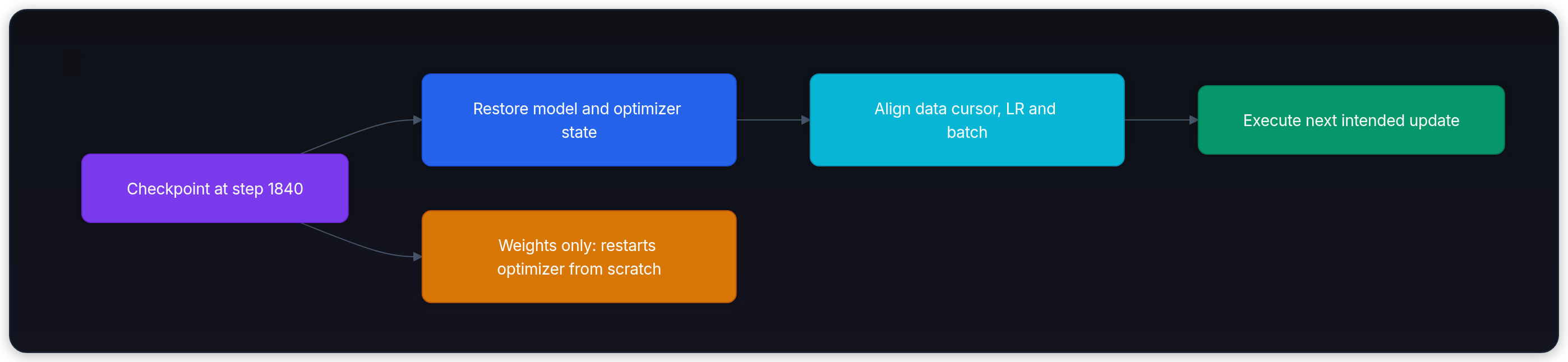
We'll use a concrete run named policy-sft-v4 to walk through every recovery boundary: four data-parallel replicas, two sequences per microbatch, eight microbatches per accumulation window, and a committed checkpoint at update 1840. The same operational rules govern full-weight pretraining and parameter-efficient fine-tuning (LoRA): which state survived, which data sample comes next, and did your replacement hardware alter the optimization trajectory?

Weights are only one part of a continuation

Training loops introduced the optimizer and scheduler. A restart must restore their internal state, not merely reconstruct the model architecture. You need to distinguish three operations before calling a checkpoint loader:

For AdamW, optimizer state includes the first and second gradient moments ($m$ and $v$) alongside parameter step counters ^{[1]Reference 1Decoupled Weight Decay Regularization.https://arxiv.org/abs/1711.05101}. For mixed precision, you must include the gradient scaler when the recipe uses one. Save per-rank random number generator (RNG) states and the data loader resumable cursor. Preserve the model, tokenizer, chat template, dataset slice, and training arguments needed to interpret them. Evaluation history helps select a checkpoint, but it isn't a substitute for optimization state.

Adapter checkpoints also require the correct frozen base weights and adapter configuration. A merged inference export isn't a resumable adapter checkpoint. Tooling frameworks distinguish intermediate training checkpoints from final exports; torchtune documents separate resume requirements for full-weight and LoRA recipes ^{[2]Reference 2Checkpointing in torchtune.https://meta-pytorch.org/torchtune/stable/deep_dives/checkpointer.html}.

Continuation isn't a guarantee of bitwise replay. A different cluster topology can change all-reduce reduction trees, random streams, and data partition assignments. Restore the intended state, document any topology changes, and compare loss trajectories against an acceptable tolerance. Exact replay demands strict control over CUDA kernels, non-deterministic operations, and sample batching.

What lost optimizer moments break

What happens when you restore weights but let AdamW start with zeroed moments? AdamW normalizes gradient steps by running second moments: $\theta_{t+1} = \theta_t - \eta_t \left( \frac{\hat{m}_t}{\sqrt{\hat{v}_t} + \epsilon} + \lambda \theta_t \right)$ Here $v$ estimates a second moment, not the variance alone. If you reset both moments and the optimizer's step counter, the first bias-corrected moments are $\hat m_1=g$ and $\hat v_1=g^2$. The adaptive gradient term moves a scalar coordinate by $\eta g/(|g|+\epsilon)$, whose magnitude is at most $\eta$. A tiny gradient doesn't make that first update arbitrarily large. This bound excludes the separate weight-decay term.

Try three gradient magnitudes with the same learning rate:

Resetting moments still discards the history that determines future direction and magnitude. Keeping an old step counter with fresh moments also changes their bias correction. Either restart can change the trajectory; neither necessarily causes a loss jump or divergence.

This scalar Adam example minimizes $(w-y)^2/2$ over a repeating target sequence. It tracks first and second moments, bias-correction steps, a step-based learning rate, and a consumed data cursor. JSON round-tripping models a serialized restart:

Even keeping the step counter doesn't reconstruct the lost moments. In a real cluster restore drill, compare the next sample IDs, current learning rate, optimizer moments, and next gradient update against an uninterrupted reference run. A smooth-looking loss curve doesn't prove mathematical continuity.

Reliability and the two checkpoint completion points

Large clusters have more opportunities for interruption. Llama 3 405B used configurations with up to 16,384 H100 GPUs. Over one reported 54-day period, the team recorded 419 unexpected interruptions and 47 planned ones; these included several kinds of hardware and software faults ^{[3]Reference 3The Llama 3 Herd of Models.https://arxiv.org/abs/2407.21783}. Those observations don't establish a universal GPU failure rate.

For a simplified model of $N$ independent devices with identical, constant failure rates, where any device failure stops the job, rates add: $\text{MTBF}_{\mathrm{cluster}} = \frac{\text{MTBF}_{\mathrm{device}}}{N}.$ Shared power, network faults, repairs, and software failures violate that model's assumptions. Measure your own run's interruption frequency and lost work rather than substituting a supposed server MTBF into a GPU-count formula.

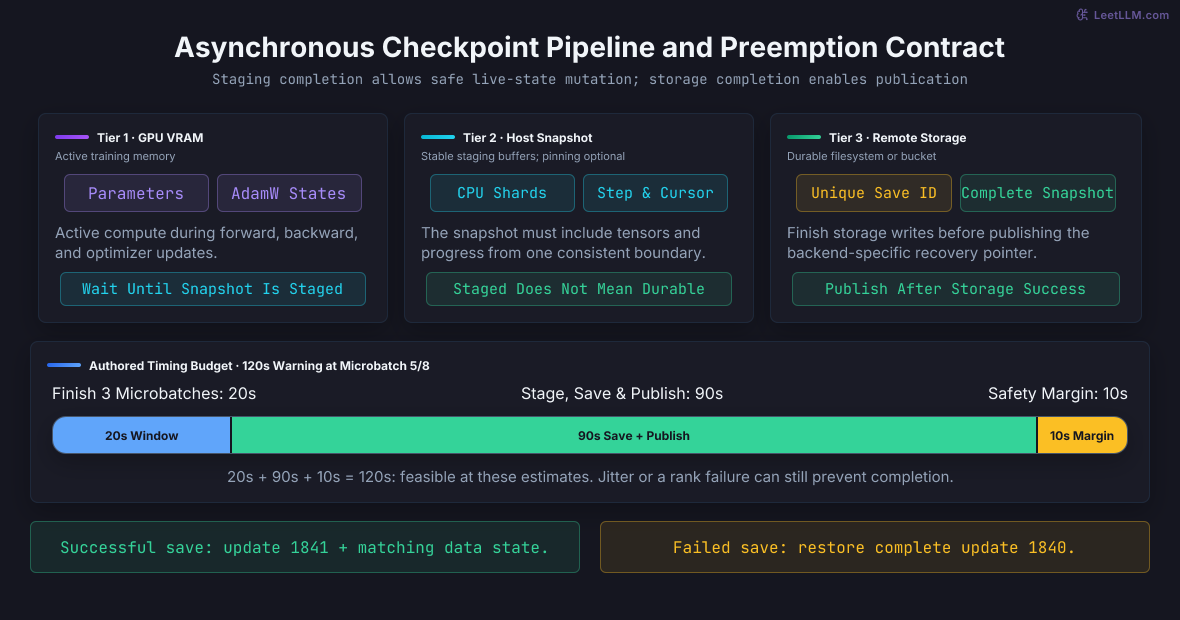
An asynchronous checkpoint separates three places where state can live:

1. Live training memory: Parameters, optimizer state, and other saved state can change as training proceeds.
2. Stable host snapshot: Staging makes a copy independent of subsequent live mutations. Pinned host buffers can improve transfer performance, but consume reserved RAM.
3. Storage: Background I/O persists the snapshot. Only successful storage completion and the required publication protocol establish a new recovery point.

PyTorch's standard async_save stages state before returning a background storage future. Its default staging can still block training. The optional DefaultStager, introduced in PyTorch 2.9, moves staging to a background CPU thread; the documented response separates staging_completion from upload_completion ^{[4]Reference 4Asynchronous Saving with Distributed Checkpointhttps://docs.pytorch.org/tutorials/recipes/distributed_async_checkpoint_recipe.html}.

Wait for staging before modifying any live state whose copy is still pending. Parameters aren't the only concern: forward passes can change buffers, and the next batch can advance RNG or loader state. Capture progress metadata at the same boundary as the tensors. Wait for storage completion before publishing or deleting the previous recovery point. Bound concurrent saves, propagate future exceptions, and close the stager when finished ^{[5]Reference 5Distributed Checkpointhttps://docs.pytorch.org/docs/stable/distributed.checkpoint.html}.

Asynchronous I/O can overlap computation, but still competes for host memory, CPU time, and storage bandwidth. Measure staging latency, storage latency, and training throughput together; there is no fixed “100 GB in three seconds” guarantee.

Atomic manifest publishing and data cursor alignment

Use a new checkpoint identifier for each save. Keep the previous committed snapshot until the new shards, framework metadata, and application state have completed successfully. A manifest should identify one consistent boundary and the expected artifacts, with integrity information such as sizes and hashes. Directory existence or a .tmp suffix alone doesn't prove completeness.

Publication depends on the storage backend. On a suitable filesystem, an atomic rename can replace a pointer file after the checkpoint completes; crash durability also requires the relevant file and directory synchronization Linux fsync documentation. An object store doesn't provide a transaction over an arbitrary collection of shard uploads. For Google Cloud Storage, individual object writes are atomic; a generation-match precondition can protect a latest pointer update from competing writers ^{[6]Reference 6Cloud Storage Consistency: Atomic Operationshttps://docs.cloud.google.com/storage/docs/consistency [7]Reference 7Cloud Storage Request Preconditionshttps://docs.cloud.google.com/storage/docs/request-preconditions}. Publish that pointer only after its referenced checkpoint is complete, and validate the checkpoint when loading.

A clean weight restore still fails if the data position describes a different boundary. A recorded consumed batch count plus a deterministic sampler can suffice for a simple replayable dataset. A worker's prefetched producer position can be ahead of what training consumed. Stateful streaming, random transforms, and packing may need worker RNG, sampler, dataset, and buffered-example state as well.

TorchData's StatefulDataLoader supports state_dict and load_state_dict; its default strategy tracks yielded batches and fast-forwards, while stateful datasets and samplers can provide their own restore state. It aggregates state across workers, not across distributed ranks ^{[8]Reference 8TorchData Stateful DataLoaderhttps://meta-pytorch.org/data/main/torchdata.stateful_dataloader.html}. A topology change therefore needs an explicit data-partition policy, alongside tensor resharding.

Preemption is a strict deadline, not a save command

Suppose update 1840 is durably committed to storage, and a preemption warning signal (such as a cloud spot termination notice or a cluster scheduler SIGTERM) arrives after microbatch 5 of the next 8-microbatch accumulation window.

Your training policy saves only at completed optimizer boundaries. There are two valid operational outcomes:

1. All nodes remain healthy and there's enough time to complete the remaining 3 microbatches, perform the optimizer step, stage the checkpoint to host RAM, and update the manifest for step 1841.
2. Time runs out or a rank dies abruptly. The orchestrator terminates, discards partial in-flight state, and reboots from durable step 1840. In this illustrative run, every update consumed 64 examples and none was skipped, so the saved global consumed-example count is $1840\times64=117{,}760$. That count isn't itself a dataset row ID or byte offset.

Never pair weights from step 1840 with a data cursor that advanced past microbatch 5. That mistake silently drops those five microbatches without applying their gradients. Mid-window recovery needs the in-flight accumulated gradients, accumulation counter, matching scaler, model buffers, RNG, and data state. With AMP, those gradients may still be scaled; preserve their representation and keep the scale constant throughout accumulation ^{[9]Reference 9Automatic Mixed Precision Exampleshttps://docs.pytorch.org/docs/stable/notes/amp_examples.html}. Unless your framework explicitly supports and tests that recovery, use completed update boundaries.

Signal handlers should only set an internal shutdown flag, not initiate distributed network I/O. The main loop coordinates the save at a clean boundary. If a member of an ordinary fixed process group dies, collectives can't complete normally; a fault-tolerant launcher must recover or reconfigure the job. Periodic durable checkpoints remain necessary because not every failure gives a warning.

Budget the entire remaining path

A 90-second checkpoint doesn't fit into a 90-second warning if you also need to finish active microbatches and publish manifests. The preemption budget equation is: $T_{\mathrm{warning}} \ge T_{\mathrm{window}} + T_{\mathrm{save}} + T_{\mathrm{margin}}$ Here $T_{\mathrm{save}}$ includes time through durable publication, and $T_{\mathrm{margin}}$ absorbs network and disk jitter:

A blocking save every five minutes of compute spends 23.1% of cluster wall-clock time writing files under these authored timings. Increasing the compute interval to twenty minutes drops that fraction to 7.0%, but increases work exposed to failure. With asynchronous saving, work performed while a snapshot uploads is also uncommitted until publication. Choose the interval using measured latency, interruption frequency, and acceptable replay cost. The warning calculation establishes feasibility at the estimates, not a deadline guarantee.

Sharded saves need a compatible restore path

FSDP and ZeRO-3 distribute persistent parameters and optimizer state rather than keeping a complete copy on every GPU ^{[10]Reference 10ZeRO: Memory Optimizations Toward Training Trillion Parameter Models.https://arxiv.org/abs/1910.02054}. FSDP can temporarily all-gather a module's weights for computation. For checkpointing, ask two questions: did the save complete reliably, and can the restore loader interpret its layout?

A full state dictionary can gather tensors onto one rank, possibly into host memory. For 70 billion parameters, BF16 weights occupy 140 decimal GB; each FP32 Adam moment occupies 280 GB. Two moments plus those weights total 700 GB, before any separately saved master weights or other state. Consolidation needs enough capacity at its destination and substantial transfer time; it isn't automatically an instant GPU OOM if the framework offloads to a sufficiently large host.

PyTorch Distributed Checkpoint (DCP) can save local shards without first constructing the entire tensor on one rank ^{[11]Reference 11PyTorch Distributed Checkpoint (DCP) Recipehttps://docs.pytorch.org/tutorials/recipes/distributed_checkpoint_recipe.html}. Its metadata describes parameter identities, global tensor properties, and shard coordinates. The storage path can stage tensors through CPU memory; “distributed save” doesn't imply a direct GPU-to-object-store transfer.

Resharding across topologies without single-node bottlenecks

When you intentionally change the partitioned layout, the loader must map saved coordinates into the new layout. Not every model-parallel mesh permits every world size: check divisibility, parameter identities, and the framework's supported model and optimizer mappings.

Under DCP, resharding happens without central gathering:

1. Initialize compatible destination model and optimizer state dictionaries, with tensors allocated in the target distributed layout.
2. Each destination rank consults the shared .metadata index file.
3. Each rank calculates which source shard files intersect its assigned tensor slice.
4. Distributed readers load the relevant serialized data and copy the required logical slices into destination tensors.

DCP's PyTorch 2.14 filesystem reader loads a serialized tensor into CPU memory and then narrows it to the requested slice. Logical slicing therefore doesn't guarantee reading only the corresponding value bytes or allocating only the destination slice ^{[12]Reference 12PyTorch 2.14: Distributed Checkpoint Filesystem Readerhttps://github.com/pytorch/pytorch/blob/v2.14.0/torch/distributed/checkpoint/filesystem.py}.

DCP explicitly doesn't guarantee checkpoint compatibility across PyTorch versions, including changes within a major release ^{[5]Reference 5Distributed Checkpointhttps://docs.pytorch.org/docs/stable/distributed.checkpoint.html}. Test the actual target stack. DeepSpeed Universal Checkpointing uses a ZeRO save, explicit conversion, and Universal load; supported topology changes still require matching model parameter identities and compatible shapes ^{[13]Reference 13Universal Checkpointing with DeepSpeed: A Practical Guide.https://www.deepspeed.ai/tutorials/universal-checkpointing/}.

This small coordinate exercise reconstructs eight destination slices from four source slices and rejects gaps and overlaps. It deliberately builds a complete Python list in one process for inspection. It is not a DCP implementation or a test of distributed I/O and memory:

Keep the update size separate from the GPU count

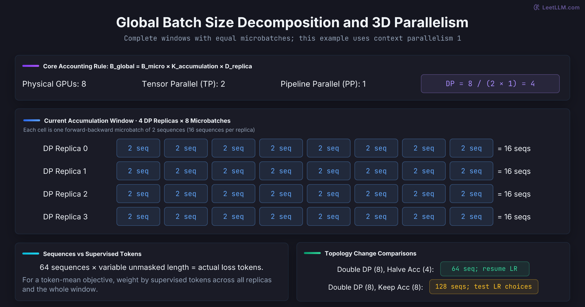
For complete accumulation windows with equal microbatch sizes: $B_{\mathrm{global}} = B_{\mathrm{micro}} \times K \times D_{\mathrm{replica}}$ Here $B_{\mathrm{micro}}$ is the sequence count per replica's microbatch, $K$ is the number of accumulated microbatches per update, and $D_{\mathrm{replica}}$ counts independent data-parallel replicas. Workers collaborating on one replica don't contribute independent examples.

For a regular mesh whose distinct axes are tensor parallelism ($\mathrm{TP}$), pipeline parallelism ($\mathrm{PP}$), context parallelism ($\mathrm{CP}$), and data parallelism: $D_{\mathrm{replica}} = \frac{N_{\mathrm{GPUs}}}{\mathrm{TP} \times \mathrm{PP} \times \mathrm{CP}}$ Context-parallel workers split one example's sequence rather than adding independent examples. This product formula isn't a universal description of overlapping expert-parallel or hybrid process groups. Eight GPUs with $\mathrm{TP}=2$, $\mathrm{PP}=1$, and $\mathrm{CP}=1$ form $D=4$ replicas. Halving accumulation while keeping $D=4$ cuts the nominal global batch in half.

Sequences versus supervised tokens and loss reduction

Sequence counts don't equal token throughput. In instruction tuning and conversational SFT, sequence packing, system prompt masking, and variable response lengths mean that two batches with identical sequence counts carry different numbers of loss-bearing tokens: $\text{Tokens per update} = \sum_{i=1}^{B_{\mathrm{global}}} \text{Length}_{\mathrm{unmasked}}(i)$ If replica 0 processes 4,800 supervised tokens while replica 1 processes 9,600, averaging their per-device mean loss values equally computes $\frac{1}{2}(\bar{\mathcal{L}}_0 + \bar{\mathcal{L}}_1)$. That naive average assigns twice as much weight to tokens on replica 0 as tokens on replica 1, distorting the true gradient.

If the intended objective is a mean over supervised tokens, use: $\mathcal{L}_{\mathrm{global}} = \frac{\sum_{r} \sum_{j} \mathcal{L}_{r, j}}{\sum_{r} N_{\mathrm{tokens}, r}}$ This is a choice of objective: a deliberately equal-weighted per-example objective is different and can be valid. For the token mean, count supervised targets after shifting and masking across the whole accumulation window and all replicas. Ordinary DDP averages gradients across replicas ^{[14]Reference 14DistributedDataParallelhttps://docs.pytorch.org/docs/stable/generated/torch.nn.parallel.DistributedDataParallel.html}. With $D$ replicas and a global token count $N$, backpropagating each replica's local loss sum multiplied by $D/N$ gives the desired gradient after that averaging. Check trainer normalization before adding any scale factor; don't also divide by $K$ when the global denominator already includes all $K$ microbatches.

Here the numbers are hypothetical scalar gradients of individual token losses. One replica has one token; another has three:

This arithmetic checks the reduction, not a running process group. Inspect your distributed trainer's real gradient normalization with a small reference batch.

Preserve the scheduler before tuning a new batch

When continuing a run at the same effective batch size, restore the scheduler phase directly. Don't restart warmup just because the process restarted.

Changing the global batch changes the optimization trajectory. Doubling tokens per update approximately halves the number of updates for a fixed token budget. Doubling sequences has that effect only if their average token contribution stays comparable.

A schedule with 100 warmup updates needs 6,400 examples at 64 examples/update and 12,800 at 128. Its milestones move to later data volumes, and a fixed data budget may end before the original step-based decay finishes. Decide whether to preserve update milestones or remap them to a data budget. Log whether the schedule uses updates, examples, or tokens.

A skipped AMP step isn't a successful update

In a standard FP16 GradScaler loop, nonfinite gradients can cause the optimizer step to be skipped. Keep separate counters for attempted accumulation windows, consumed data, and successful optimizer updates. A scheduler defined per successful update should stay fixed when no update occurred; a deliberately data-indexed scheduler follows its own policy.

Perform overflow checks and scale updates at effective-batch boundaries, keeping the scale constant during accumulation ^{[9]Reference 9Automatic Mixed Precision Exampleshttps://docs.pytorch.org/docs/stable/notes/amp_examples.html}. A skipped step can still consume data and change scaler state. Preserve both in the checkpoint. Don't infer success from scaler.step(...) returning None: many optimizers return None even after a real update. Use the framework's supported overflow handling.

Scaling rules are hypotheses to test

Goyal et al. popularized linear learning-rate scaling with gradual warmup for large-batch SGD, training ResNet-50 with batch 8,192 on 256 GPUs ^{[15]Reference 15Accurate, Large Minibatch SGD: Training ImageNet in 1 Hour.https://arxiv.org/abs/1706.02677}. The approximation compares one large step with several smaller steps while assuming their gradients change little. It can break early in training or at very large batches; it isn't an AdamW SFT guarantee.

Malladi et al. derive an Adam scaling rule from stochastic differential equation approximations under specified noise and moment assumptions ^{[16]Reference 16On the SDEs and Scaling Rules for Adaptive Gradient Algorithmshttps://arxiv.org/abs/2205.10287v3}. For a batch multiplier $\kappa$, their rule changes more than the learning rate:

$$\begin{aligned} \eta'&=\sqrt\kappa\,\eta,\\ \beta'_i&=1-\kappa(1-\beta_i),\\ \epsilon'&=\epsilon/\sqrt\kappa. \end{aligned}$$

The new $\beta_i$ must remain valid optimizer coefficients. This conditional result isn't a theorem that changing only AdamW's LR by $\sqrt\kappa$ preserves a fine-tuning run, nor that linear scaling always diverges. Compare controlled runs, including a fixed-LR baseline, and evaluate quality at a comparable data budget.

McCandlish et al. study a gradient-noise scale: $\mathcal B_{\mathrm{simple}}=\frac{\operatorname{Tr}(\Sigma)}{\lVert G\rVert^2},$ where $G$ is the mean gradient and $\Sigma$ is the covariance of individual-example gradients ^{[17]Reference 17An Empirical Model of Large-Batch Training.https://arxiv.org/abs/1812.06162}. It predicts the scale of the largest useful batch in their studied settings, rather than an exact universal threshold. Larger batches can reduce update count with diminishing returns, while increasing examples needed to reach a target. That optimization tradeoff doesn't imply linear wall-clock speedup: kernel efficiency and communication matter too.

Diagnose a symptom before choosing a recovery

A loss spike doesn't reveal its cause. Record the last known-good checkpoint, exact batch identity, token counts, learning rate, scaler state, and per-rank timings before changing the run.

A slow rank can delay dependent collectives and extend the critical path. Communication may overlap backward computation, so this isn't a literal barrier where every GPU waits throughout the whole pass. Separate compute time, rank arrival skew, and collective completion time. Compare clock event reasons with a healthy device under matched work; there is no model-independent “bad clock” threshold ^{[18]Reference 18nvidia-smi documentationhttps://docs.nvidia.com/deploy/nvidia-smi/index.html}.

Link errors and reduced bandwidth can leave a job alive but slower. Counter trends, link state, and measured throughput help distinguish fabric faults from compute imbalance. A particular rate change doesn't imply a fixed tenfold slowdown, and one counter alone isn't sufficient reason to evict a node.

The Llama 3 report recorded six silent data corruption incidents in its interruption breakdown ^{[3]Reference 3The Llama 3 Herd of Models.https://arxiv.org/abs/2407.21783}. Absence of an ECC alert doesn't rule out erroneous computation. Controlled canary computations can help identify faults, but require matched inputs, precision, kernels, and justified tolerances; ordinary floating-point differences aren't proof of bad silicon. A canary doesn't guarantee detecting every error before it affects training.

What a rollback policy must decide

Reject nonfinite training state as a new operational recovery point, and preserve diagnostic evidence. For an unexpected finite loss spike, use thresholds calibrated to the run's normal variability. A median plus three standard deviations over 50 steps is a possible authored heuristic, not an established universal training policy.

Reproduce the suspect batch from a known-good checkpoint, preferably on verified healthy hardware. Check masks, zero-token batches, learning rate, scaler behavior, and gradient norms. Use bounded retries so an automatic restart cannot loop indefinitely.

Choose how far to rewind from evidence about the first affected state. “Two checkpoints back” doesn't guarantee safety. Quarantine data only when the diagnosis supports it, with a recorded decision. Skipping examples or changing the shuffle seed changes the data trajectory; it is a deliberate new continuation policy, not exact recovery.

Choose the objective, trainable weights, and precision separately

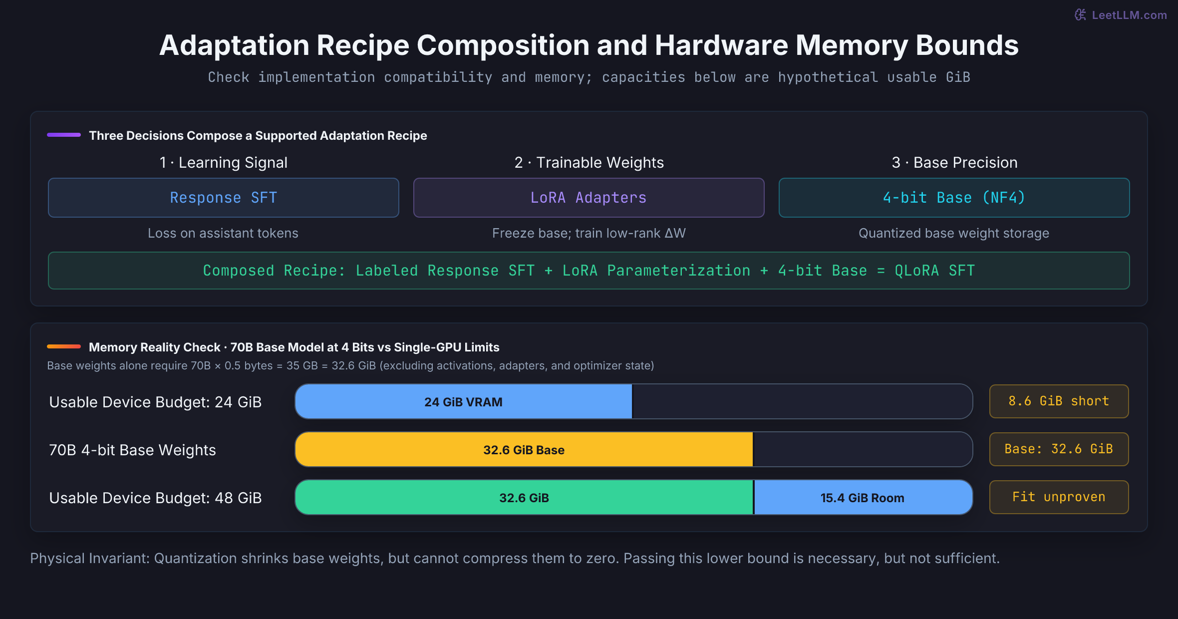
Training recipes aren't a single dropdown choice. SFT and continued pretraining define what the model learns. LoRA defines which parameters update. QLoRA adds 4-bit base-model quantization to adapter tuning. Distillation learns from a teacher, using soft targets ^{[19]Reference 19Distilling the Knowledge in a Neural Network.https://arxiv.org/abs/1503.02531} or generated sequences ^{[20]Reference 20Sequence-Level Knowledge Distillationhttps://aclanthology.org/D16-1139/}; logits aren't required for every distillation method.

These are conceptually separate decisions, but their implementations aren't freely interchangeable. Check that the architecture, quantization backend, adapter implementation, and hardware support the combination you chose.

Domain-adaptive pretraining can improve specialized comprehension, but unfamiliar vocabulary alone doesn't prove it's necessary ^{[21]Reference 21Don't Stop Pretraining: Adapt Language Models to Domains and Tasks.https://aclanthology.org/2020.acl-main.740/}. Small labeled datasets make LoRA SFT an attractive starting point, though adapters aren't guaranteed to beat full fine-tuning ^{[22]Reference 22LoRA: Low-Rank Adaptation of Large Language Models.https://arxiv.org/abs/2106.09685}.

Reject impossible memory plans before launching

The original QLoRA paper demonstrated fine-tuning a 65B model on a single 48GB GPU ^{[23]Reference 23QLoRA: Efficient Finetuning of Quantized LLMshttps://arxiv.org/abs/2305.14314}. That empirical result doesn't mean a 70B model fits within a 24 GiB usable device budget. Here 24 and 48 GiB are hypothetical capacities, not conversions of specific products' advertised GB.

At an ideal four bits per parameter, a 70B model requires: $\text{Memory}_{\mathrm{base}} = \frac{70 \times 10^9 \times 4\text{ bits}}{8\text{ bits/byte}} = 35 \times 10^9\text{ bytes} \approx 32.6\text{ GiB}$ Base weights alone exceed 24 GiB by 8.6 GiB before quantization metadata, higher-precision tensors, LoRA adapters, activations, gradients, optimizer moments, or temporary buffers.

This all-resident four-bit plan cannot fit a 24 GiB budget. Change the plan: use a smaller model, a supported lower-bit representation, sharding, or offloading. Passing the base-only check doesn't establish training fit. For the hypothetical 48 GiB budget, the remaining 15.4 GiB must cover all omitted memory, not just adapters and activations.

Rehearse the restart before the long run

Don't wait for your first midnight preemption to discover that your checkpoint loader crashes. Run a restart drill on small test jobs:

• Local state continuity: Compare five uninterrupted steps against five steps resumed from an intermediate checkpoint. Verify that weights, Adam moments, learning rates, and data sample IDs match within floating-point tolerance.
• Distributed topology restoration: Save on four GPUs, then load on a supported target layout with eight GPUs (or another valid size). Verify model and optimizer resharding, data partitioning, and peak restore memory.
• Preemption deadline drill: Send kill -TERM <training-pid> to your test job. Exercise both a warning that fits the measured path and one that doesn't. Force an interruption during saving and verify that the loader selects the previous complete checkpoint.
• Diagnostics and recovery policy: Inject a controlled straggler or nonfinite test batch. Verify that monitoring identifies the symptom, unsafe state isn't published, retries are bounded, and any rollback or quarantine follows the configured policy.

Distinguish between your latest resumable checkpoint and your best evaluation checkpoint. Step 1840 might be your operational recovery point, while step 1600 holds your highest validation score. Store both with explicit metadata tags.